L11 - Decision Making with Markov Models

Reliability Engineering:

The discipline to develop methods and tools to evaluate and demonstrate the reliability, maintainability, availability, and safety of components, equipment, and systems.

Reliability Engineering: Field that develops methods/tools to check and prove reliability, maintainability, availability, and safety of systems.

Reliability:

Probability that the required function will be provided under given conditions for a given time interval.

Reliability: Probability that a system performs its required function under given conditions for a given time.

Safety:

Ability of the item to cause neither injury to persons, nor significant material damage or other unacceptable consequences.

Safety: Ability to avoid harm to people or significant material damage.

Reliability Engineering – Common failure distributions

• Exponential distribution:

  • For constant failure rates (random failures, e.g., electronics).

  • Formula: F(t)=1−e^−λt

  • λ = failure rate.

• Weibull distribution:

  • Flexible, models different failure behaviors (matches parts of bathtub curve).

Reliability calculation for multiple components

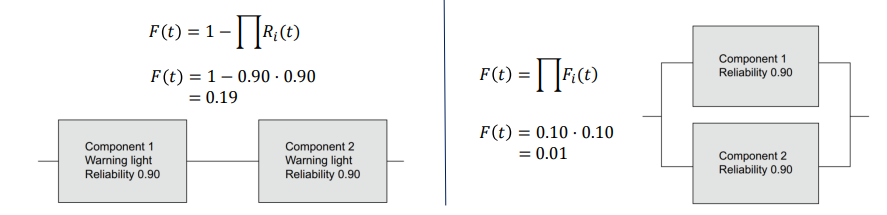
• Series configuration:

  • Example: Hydraulic circuit.

  • If one component fails → whole system fails.

  • Logical OR.

  • Example: Two components each with 0.90 reliability → System failure probability = 0.19.

• Parallel configuration:

  • Example: Aircraft engines.

  • Redundancy improves reliability.

  • Logical AND.

  • Example: Two components each with 0.90 reliability → System failure probability = 0.01.

System reliability models (overview)

• Reliability models combine component failure probabilities to estimate RAMS (Reliability, Availability, Maintainability, Safety).

• Common models:

  • Part Count Method

  • Reliability Block Diagram

  • Fault Tree Analysis

  • Reliability Graph

  • Petri Nets

  • Markov Models/Processes

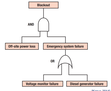
Fault Tree Analysis (FTA)

Tool for modeling failure dependencies in multi-component systems (tree structure).

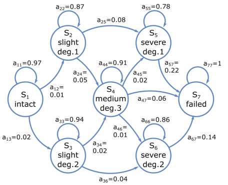
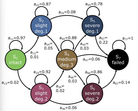
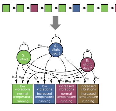
Markov Models

State-based system representation

• A system can be in one of N states at any time (e.g., intact, slightly degraded, severely degraded, failed).

• From the current state, it either:

  • Moves to another state, or

  • Stays in the same state.

• Each state is directly observable.

• The transition probabilities (numbers on arrows) show the likelihood of moving between states at each time step.

Markov Models

Deriving State transition probabilities

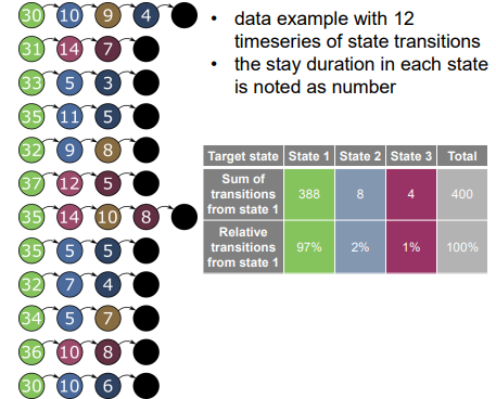
• Shows how transition probabilities are calculated from observed data.

• Example: 12 time series of state transitions are recorded.

• For each state, we count how many times the system moved to other states → Then calculate percentages.

• Table example: From State 1, 97% of the time it stays in State 1, 2% goes to State 2, 1% to State 3.

Markov Models

Predicting States into the future

• Markov model tells how future states depend only on the current state (for first-order Markov).

• Transition probability: a_ij

• If you know the initial state probability, you can model the whole process.

• The time spent in a state follows an exponential distribution, with formula: Pi(d)
  where a_ii is the probability of staying in the same state.

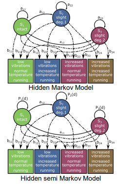
Hidden Markov Models

• In HMM, states are often not directly observed.

• Only sensor measurements are available.

• Observations (e.g., vibrations, temperature, running status) give clues about the hidden state.

• Extension of Markov Model:

  • Observations are probabilistic functions of states.

  • True states are hidden.

Hidden Markov Models

Observation based state probability

• Extension of Markov Model:

  • Observations are probabilistic functions of states.

  • True states are hidden.

• HMM defined by:

• A: State transition matrix (a_ij​)

• π: Initial state probabilities

B: Emission matrix (b_jk = P(v_k∣S_j) → Probability of observation v_k given state S_j

• N: Number of states

• Full parameter set: λ=(A,B,π,N)

Three main training problems for HMMs:

1. Find P(O∣λ)P(O | \lambda)P(O∣λ): Probability of observation sequence (Forward step).

2. Find best state sequence QQQ for observations (Backward step).

3. Adjust parameters (A,B,π,N) to maximize P(O∣λ) (Baum–Welch algorithm).

• Forward–Backward algorithm is the core method.

HMMs are widely used in:

• Speech recognition (25%)

• Human activity recognition (25%)

• Bioinformatics (19%)

• Musicology (9%)

• Tool wear monitoring (9%)

• Data processing like handwriting recognition (7%)

• Network analysis (6%)

Example: Speech recognition, gesture recognition, gene sequencing, predicting melodies.

Hidden Semi Markov Models
Time-dependent presence probability

• In a standard HMM, time spent in a state follows an exponential distribution:
  P_i(d)
  where a_ii​ is the probability of staying in the same state.

• In HsMM, instead of a fixed self-transition probability, we use a duration density P_i(d) that can be adjusted.

• Other distributions (Gaussian, Gamma, etc.) can replace exponential.

• HsMM parameters: λ=(A,B,π,D,N)

  • D: Duration matrix containing P_i(d) for each state.

Required inputs for AG

• Engineering expertise needed:

  • Failure modes & mechanisms knowledge.

  • Suitable failure indicators.

  • Proper sensors & acquisition setup.

• Data required:

  • Run-to-failure data, labeled anomalies.

• Scope & user analysis:

  • Understand user goals, connected systems, automation level.

Epistemic (structural) Uncertainty:

Epistemic uncertainty is due to a lack of knowledge about the behaviour of the system that is conceptually resolvable.

• Comes from lack of knowledge about system behavior.

• Can be reduced with more study and expert judgment.

Aleatoric (statistical) uncertainty:

Aleatory uncertainty arises because of natural, unpredictable variation in the performance of the system.

• Comes from natural, unpredictable variations.

• Cannot be reduced by expert knowledge.

• Also called irreducible uncertainty.

Visualization formats

Circular bar chart:

• Pro: Shows degradation and failure probability.

• Con: Only shows current time, not RUL; uneven bar length may cause misperception.

Component model:

• Pro: Clear mapping to components.

• Con: Only shows current time; high visualization effort.

Network diagram:

• Pro: Many systems/components; shows degradation & probabilities.

• Con: Only normalized data; comparability issues due to radial layout.

Line chart:

• Pro: Shows history and trends; can combine prognosis & diagnosis.

• Con: Becomes cluttered with many systems.

Key Findings

• Reliability engineering uses statistical analysis of past failure data; data analytics helps to understand real system health.

• Failure rates of single components can be combined statistically to model complex systems.

• Reliability engineering and PHM have differences, similarities, pros, and cons — PHM especially adds feedback through data analysis.

• In Markov Models, state-to-state interactions are described by transition probabilities.

• Hidden Markov Models extend this by linking states to probabilistic observations.

• Machine learning & prognostics can support operators’ decision-making via automated onboard data processing.

• Even with low structural uncertainty (large databases), statistical uncertainty must be considered.

• PHM system requirements differ for different users and can be met via visualization techniques and specialized IT infrastructure.