Introduction to Machine Learning

FS2026

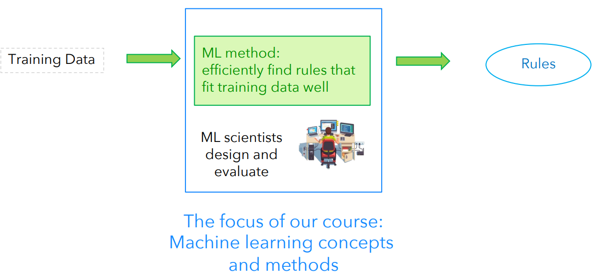
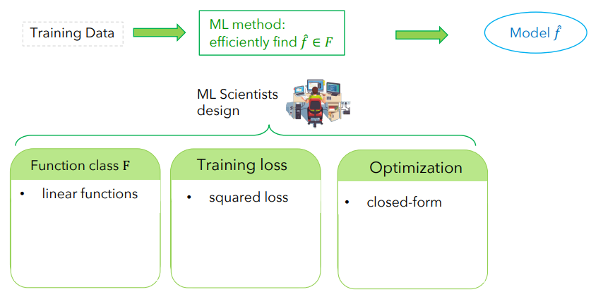
Simplified diagram of machine learning

Supervised Learning - Definition

Learning with training data that contains inputs together with correct outputs (= labels). The Goal here ist to predict the correct output.

Unsupervised Learning - Definition

Learning with training data that contains only inputs and no labels. The Goal here is to discover useful structure in the data.

Examples of supervised learning:

Classification, Regression, Structured prediction

Examples of unsupervised learning

Clustering, Anomaly detection, Dimensionality reduction, Generative Modeling

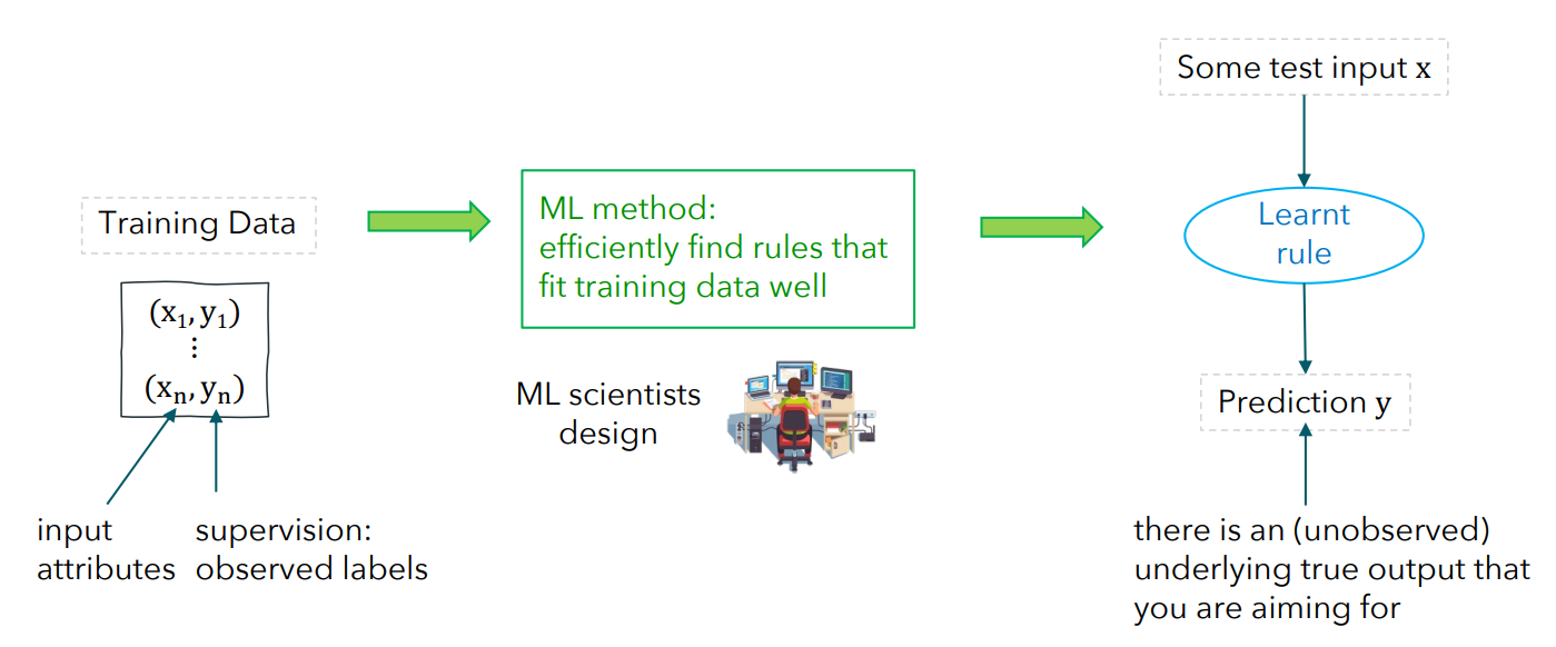
Simplified diagram of supervised learning:

Prediction y can also be called y^, or f^(x)

Simplified diagram of unsupervised learning:

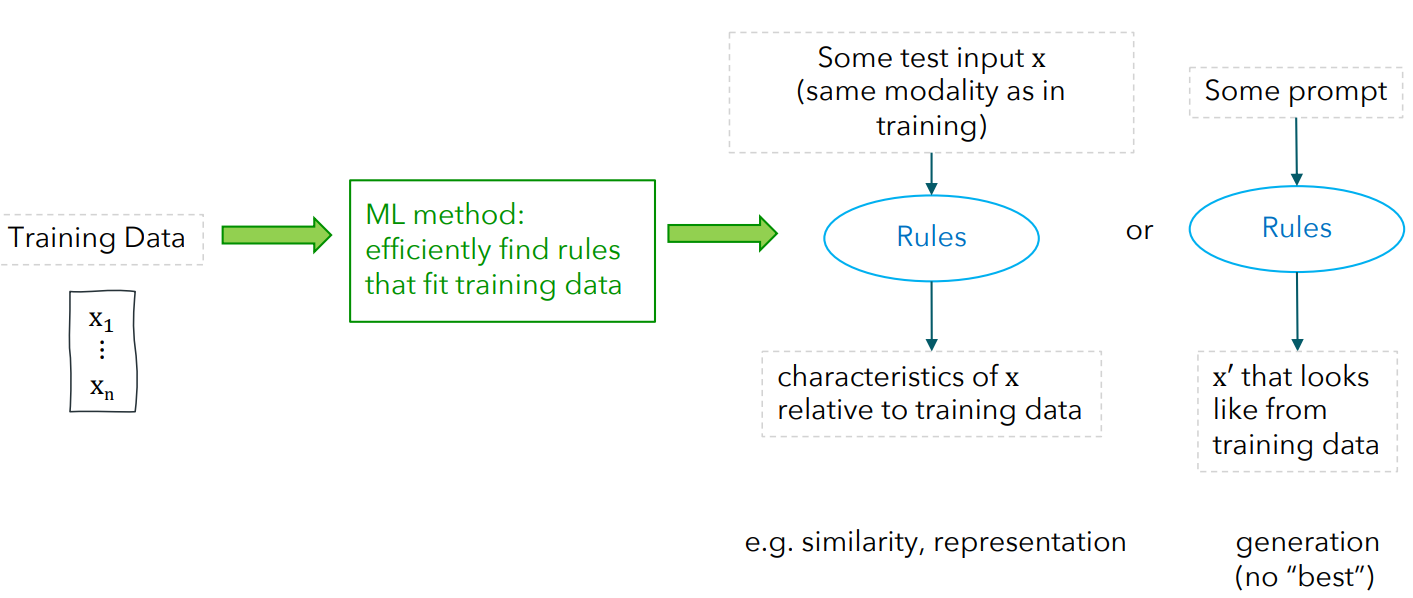
Goals of unsupervised Learning: 2 concepts

1) Describe new input x relative to training data (is it similar, is it an anomaly?, etc.)
2) Generate new data x’ that looks similar to training data (Generative modeling)

Machine Learning Pipeline for linear Regression

Linear Regression is always linear functions, squared loss, closed-form, no matter the dimension

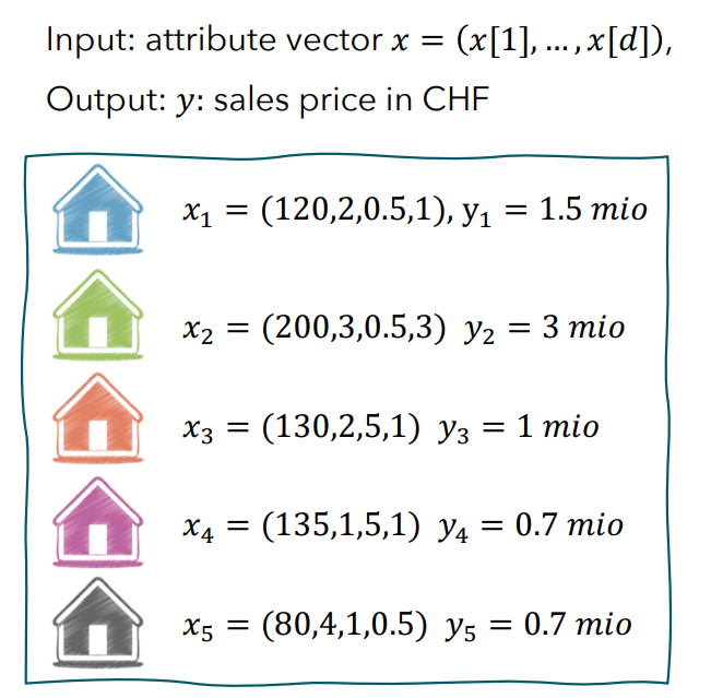
Difference House Prices (Linear Regression) example between 1 Dimension and d Dimensions

1D: We only have one attribute x (x is 1D) → E.g. x = (size)
dD: We have d attributes → x is dD → E.g. x = (size, #bathrooms, …, years since construction)

How can the linear function class be represented in 1d?

Linear function equation:

f(x) = w0 + w1*x with w0: y-Achsenabschnitt, w1: Steigung

Linear Regression:

Function Class F: Linear Functions

Training Loss L: Squared Loss

Optimization: We can use closed Form solution

Characteristics of different Losses: Squared, Huber, Asymmetric

Squared Loss: Symmetric → Overestimation and Underestimation are treated equally, large penalty on outliers (because grows quadratically)

Huber Loss: Ignores outliers

Asymmetric Losses: Weigh over- and underestimation differently

Feature Vector x in 1D:

X = (x1, …, xn) mit x1, …, xn 1D

E.g. x_i = (size)

Feature Vector x in dD:

X = (x1, …, xn) mit x1, …, xn dD

E.g. x_i = (size, #bathrooms, …, years since construction)

Linear Regression Closed Form:

w = (X^TX)^(-1)X^Ty

What changes if we use nonlinear regression?

Function Class F: We can use nonlinear functions

Optimization: Gradient Descent can be used (it’s always used when there is no closed form or closed form is computationally expensive)

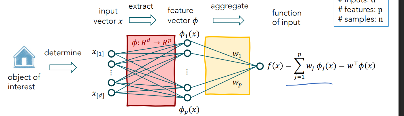
General Form of nonlinear functions in ML Pipeline:

Some ML models have fixed phi (linear regression, kernel regression, etc.), phi maps d dimensions (from input) to p dimensions

Nonlinear in x, linear in phi

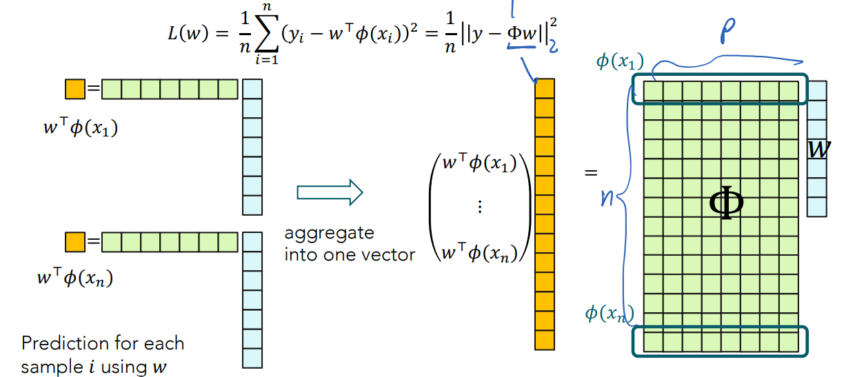
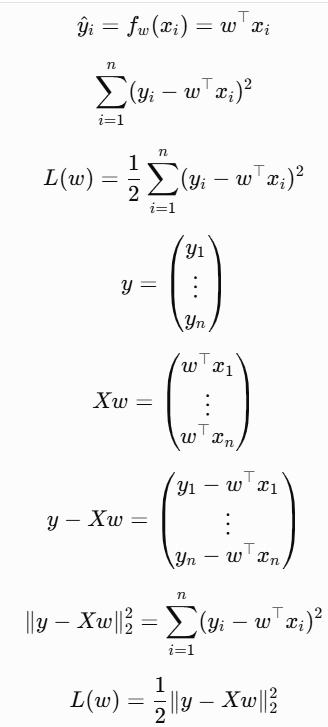
Matrix notation of loss L(w) of nonlinear function (also squared loss)

Why can/can’t we use closed form for nonlinear functions?

We can use it, we only have to replace X matrix with Phi matrix.
Problem: Phi^TPhi can have a high computational cost to compute and there is a lack of generality for different losses (other than squared loss)

→ That’s why we need gradient descent

What do we use Gradient Descent for?

It’s a general iterative algorithm to minimize our loss L(w) and thus find out our weight vector w for our model f.

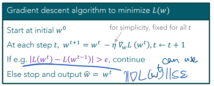
Gradient Descent in 1D: 1. In which direction do we move? 2. How far in that direction? 3. When should we stop?

1. In direction of sign of negative derivative at w_now

2. nü~ = nü*|L’(w_now)| → In direction of nü

3. Stop when it can’t improve much anymore, so for example when: |L(w_now) - L(w_previous)| <= epsilon

What changes when we execute Gradient Descent in nD than in 1D?

For minimizing L(w) we have multiple directions in which to go to. → We need gradient (because gradients point in direction of steepest descent)

Geometric Intuition of contour lines in relation with Gradient Descent:

• Steepest direction is orthogonal to contour lines

• Direction of steepest increase: ∇L(w)

• Direction of steepest decrease: -∇L(w)

What does hold on contour lines?

On those lines the loss has the same value.

Gradient Descent algorithm:

True or False: We can use machinery from linear regression to solve regression in nonlinear function spaces by just replacing the data matrix 𝑋 by the feature matrix Φ

True

How can we rewrite the Squared Loss in matrix notation?

Which of the following statements are true?
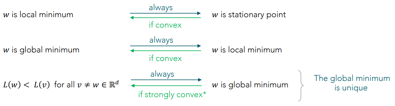
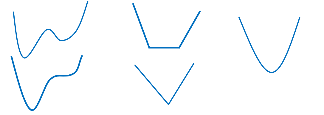
(A) All convex functions have only one local minimum that is a global minimum
(B) For convex functions, all stationary points are local minima
(C) For convex functions, all stationary points are global minima

(B) and (C) are true immediately if you plug in ∇𝐿 𝑤 = 0 in first order condition

Relation Convexity and global/local minima

Why does Gradient Descent work for linear Regression?

Because linear Regression with squared Loss is a convex problem. Convergence is only guaranteed for the convex case. (otherwise we can get stuck in local minima or diverge to infinity)

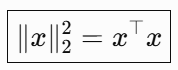
What holds for the 2 norm squared?

What is Conditioning?

It tells us how nicely shaped the loss landscape is. If the contour lines (= same loss values) are more spheres we have a well conditioned case, and if they are more ellipses we have an ill conditioned case.

Well-conditioned case of GD?

λmax ​≈ λmin​, contour lines are almost circles, loss equally steep in all directions, GD works

Ill-conditioned case for GD

λmax​ » λmin, contour lines are stretched ellipses, one direction very steep, the other flat → small stepsize: slow in flat direction, large stepsize: oscillations in steep direction
→ Solution for ill-conditioned case → use Momentum/accelerated methods​

Momentum/accelerated methods to find minima:

Momentum speeds up flat directions, speeds up GD (Gradient Descent)

Why SGD (Stochastic Gradient Descent)?

It uses a different loss than GD (not gradient over all points but only on a random subset of points, which is called mini batch with batch size |S|). This saves memory, when the batch size is smaller than n
→ works because minibatch gradient is correct on average (Expectation value)

Full batch GD, Original SGD, Minibatch SGD?

Full batch: |S| = n, Original: |S| = 1, Minibatch: 1 < |S| < n (Full batch = normal GD)

Effect on batch size in SGD?

|S| small → cheap but noisy, but this can sometimes also escape saddle points

|S| large → expensive but stable (closer to GD, can more and more get stuck in stationary points)

What is convexity? Explain with the 3 conditions.

Function is convex if it has a “bowl shape”.

0-th order condition: Real function always below linear connection of two random points.

1-st order condition: Tangent of two points always below function.

2-nd order condition: Curvature is always non-negative .

What is strong convexity?

Stronger than convexity. It holds: strong convex → unique global minimum, It means that the loss landscape is curved enough so that there is only one best solution.

Characterize the following functions:

Training Loss, Generalization Error and Estimation Error?

Training Loss: Measures error on trainings data D. L(f;D)

Generalization Error: Measures expected error on new data. L(f;P) (P is the joint distribution that we assume our test data is drawn from and our trainings data is randomly sampled from)

Estimation Error: Measures how far the learned model is from the ideal model f*.

Linear Regression, what underparametrized case, overparametrized case and n=d mean for the errors and amount of solutions for our problem.

Underparametrized n>d: More samples than parameters, if we increase n our model sees more data and thus the effect of noise gets averaged out, Estimation Error shrinks, usually unique solution

Overparametrized n<d: More parameters than samples, More DoFs than constraints from Data → infinitely many solutions, Training error can be zero, b.c. we can fit data perfectly

n=d: Possibly a unique solution

Main Message: More samples usually help, but in high dimensions (n<d) many different models can fit the training data perfectly, and not all of them generalize well.

Definition Model complexity

means how flexible the function class F is. F0 = constant functions, F1 = linear, F2 = quadratic, etc.

Higher model complexity → more flexible functions → Fit data better → Training error shrinks

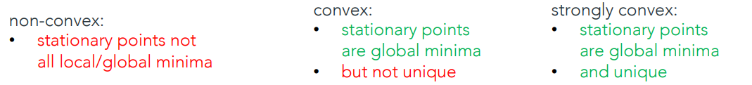
Definition Underfitting

Model is too simple and can’t capture the true relationship.

Definition Overfitting:

Model is too complex and fits random noise in training data.

Overview: Relationship model complexity vs. Training/Generalization Error

Sources for generalization error:

Bias, Variance, Irreducible noise

→ Important: Generalization Error can exist without noise because of Bias and Variance, from not being able to fit the function (bias) and/or from seeing only few samples (Variance)

Bias-Variance tradeoff in choosing model complexity

Simple Models: High Bias, Low Variance

Complex Models: Low Bias, High Variance

Good Models: Balance

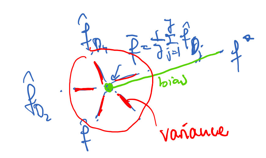
Definition Bias and Variance with pictures in mind

Bias: Distance between average over all different models for different data sets D1, D2, .. and ideal model f*

Variance: Summarized Distance between individual models fD and average over all models.