Unit 2 - Modeling Distributions of Data

pth percentile

percentage of observations at or below a given observation 

_{^{^can either choose to include the chosen value or not! ex) 2, 2, 5, 5, 6, … and looking for percentile of value 5, can count 2, 2, 5, 5, 6, … OR 2, 2, 5, 5, 6, … → both are correct!}}

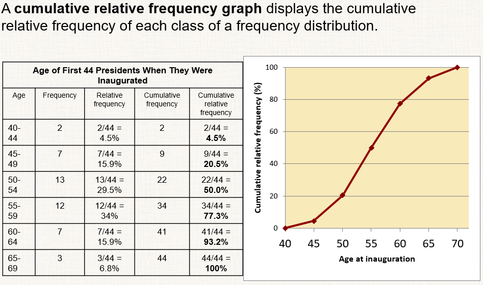
cumulative relative frequency graph

displays the cumulative relative frequency of each class of a frequency distribution

_{^{^think of y-axis as percentile}}

_{^{^go to next class → cumulates, add up percentage for that class and the ones below it}}

z-score

how many standard deviations from the mean an observation is

^ z = (observation - mean)/standard deviation

_{^{*aka standardized score}}

_{^{^higher - more above avg}}

*allows comparison of different data sets (ex: SAT vs. ACT scores, who did better on their respective test (comparing w/in their group!))

*higher z-score means more above the mean/did ‘more’ better than others, but does not mean higher # of smth (b/c z-score says nothing abt sample size!)

adding/subtracting to transform data

• add ‘a’ to/subtract ‘a’ from measures of center & location (mean, median, quartiles, percentiles) 

• shape/spread do not change _{^{(the rest change) (explanation: adding/subtracting a constant from each observation in a distribution does not change the spread)}}

multiplying/dividing to transform data

• multiply/divide measures of center & location (mean, median, quartiles, percentiles) by ‘b’

• mult/divide measures of spread by |b|

• shape does not change (unless b is negative) _{^{(the rest change)}}

!!! more unusual if percentile is farther from median (50th percentile)

Q₁ 25th percentile, Q₃ 75th percentile

write units

cumulative rel freq graph, what will be the shape of histogram -> look at where the median is, if it is more left prob right-skewed, if more right it is prob left-skewed

make histogram from cumulative rel freq graph:

• x-axis same, make the gaps the bins

• y-axis is percent, make bars as tall as the change in cumulative rel freq from the graph (if looking at btwn 10-20 and 10 is 8 and 20 is 30, then the change is 22, so that is the height of the bar on the histogram!!)

density curve

a curve that is always on or above the horizontal axis and has a total area of 1 below the curve

^mean μ = at ‘balance point’

^standard deviation σ

^median = point where ½ data is above and ½ is below

_{^{*describes overall pattern of a distribution; ideal description of a distribution of data}}

_{^{*excludes outliers; not perfect}}

normal curve

• describes a normal distribution

• always same shape (symmetric, unimodal/1 peak, bell-shaped)

• completely described by its mean/standard deviation

• mean and median equal to each other and in the center of the normal curve

_{^{*since its symmetric, the mean is the avg of the endpoints (or any endpoints that are both equally away from the center like 10th and 90th percentile)}}

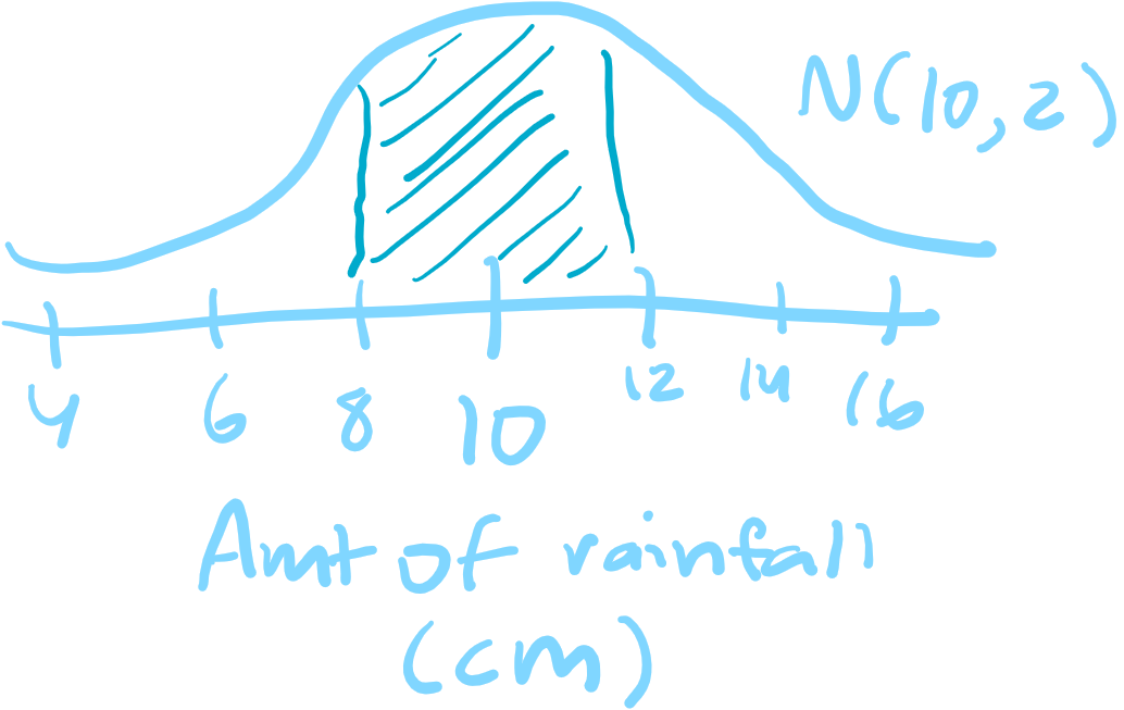
normal distribution

• described by a normal density curve

• notation: N(μ, σ)

• _{^{standard deviation is the distance from the mean to the change-of-curvature points on either side}}

68-95-99.7 Rule

68% of observations fall within 1 standard deviation (σ) from the mean

95% of observations fall within 2 σs

99.7% of observations fall within 3 σs _{^{(0.3% left, 0.15% on both sides)}}

standard normal distribution

the normal distribution has a mean of 0 and standard deviation of 1 (same units!)

standard normal table A

table of areas under the standard normal curve

^only used for z-scores/normal distributions _{^{(connects z-scores and percentiles)}}

^rows are ones and tenths place, columns are hundredths

^using it helps you find the proportion of observations BELOW the given # (like z < [given])

• ex) z-score 1.1, get 0.4 -> 40% data is below z-score 1.1 (aka percentile)

• If you want to find above (z > [given]), do 1 minus the # you get from the table

• if a < z < b, find the difference (do the value you get for b (what's on the table) minus the value you get for a, no doing any '1 - [value you get]')

• working backwards - given percentile -> convert to decimal (if '#% of all observations are GREATER than z,' do 1 - [the decimal]), find on table, look at what z it is by its row and column!

!!!

normal curve → mean = median

• if a curve is skewed, the mean is pulled towards the tail of the data

peak of the curve is the mode

-

median location on boxplot/density curve/histogram -> if skewed, half the data is still on the left and the other half is on the right. The 'shorter' part just means that the data has less variation (more condensed between values), while the 'longer' part means that there is more variation (more spread out between values). BOTH SIDES STILL HAVE THE SAME # OF DATA VALUES THOUGH!!! (same w/ quartiles, which help split data into quarters)

-

seeing what percent of values fall within 1/2/3 standard devs -> w/ mean and standard deviation, get the range for w/in 1 standard dev. Count the values that fall within the range and put it over the total to get the %. Do for each.

normal probability plot

shows if a distribution is relatively normal or not 

^x = numerical value, y = z-score _{^{(z-score vs. value graph)}}

^on calc w/ 2nd + y (stat plot) → the last graph choice

^looks linear = indicates Normal 

^systematic pattern showing not linear = indicates non-Normal distribution

*outliers appear as points far away from the overall pattern of the plot 

!!!

# means a numerical value. ex) looking at 'how many days it takes for a tulip to grow,' might get in a question '121 days'

2nd+vars (distribution) to get normalcdf and invNorm

^ONLY USED FOR NORMAL DISTRIBUTIONS, ONLY USE NUMERICAL VALUES NOT Z-SCORES!!!!!!!! USE TABLE A FOR Z-SCORES!

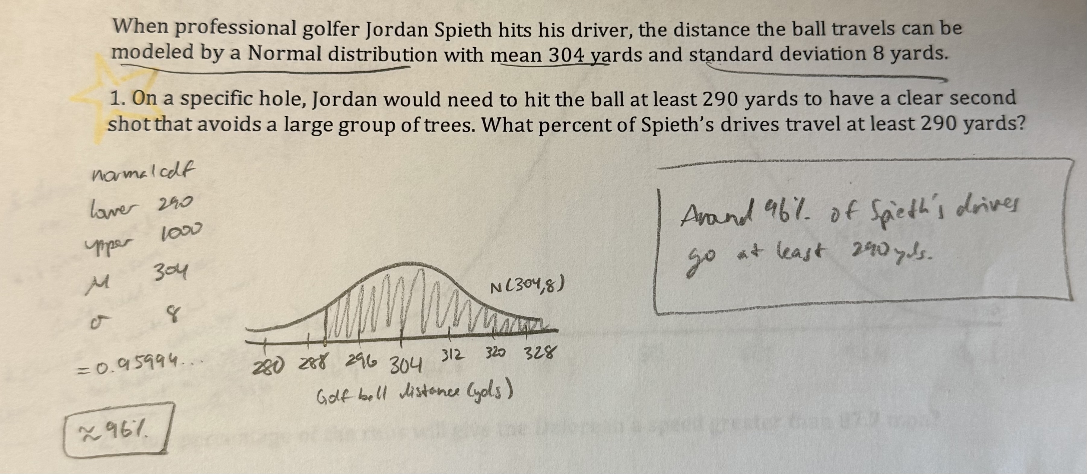
➢given a # or #s, find percentile/percent/probability/proportion - use normalcdf

-percentile: lower is negative big # (ex: -1000), upper is the given #

-percent above: lower is given #, upper is big # (ex: 1000)

-percent of [variable thing] btwn two given #s: lower is the lower #given , upper is the upper # given

^gives a decimal, that is the probability aka the percentile but as a decimal

➢find # given percent/percentile do invNorm

-bottom % -> area is the percent given but as a decimal, tail is LEFT b/c BELOW

ex) 70th percentile, area = 0.7, tail left b/c percentile talks abt numbers below a given observation

-upper # -> area is the percent given but as a decimal, tail is RIGHT b/c ABOVE

ex) looking for 20% highest values, area = 0.2, tail is right b/c looking at the 'upper' #s

What to include when drawing a normal curve (draw for each question _{^{UNLESS given a curve and you need to answer multiple questions about the same curve}})

• draw horizontal line + curve

• name of curve -> N(μ, σ)

• write #s (mean, #s related to the question, increments/scaling using standard dev, label all ticks)

• shade appropriate area btwn #s

• label what the curve represents (include units)

!!! test/question answering tips

-show work → write calculations, write down what you put into your calculator, draw curves, write sentence answers at the end!

-use #s for explanations

<-EXAMPLE PIC

!!! 

find z-score and percentile of a given observation value

find z-score (value-mean/StDev), to find percentile just use table A! (not calculator)

OR

• _{^{given that Y (# of observations that are above E (the given observation))}}

  • _{^{z-score = (E - mean)/StDev}}

  • _^percentile

    • _{^{Total observations - Y = A (value of how many are below E)}} 

    • _{^{A/Total observations = proportion}} 

    • _{^{proportion x 100 = percentile}} 

• _{^{given E’s place (nth place)}} 

  • _{^{z-score = (E-mean)/StDev}} 

  • _^percentile 

    • _{^{n/Total observations = proportion}} 

    • _{^{proportion x 100 = percentile}} 

-

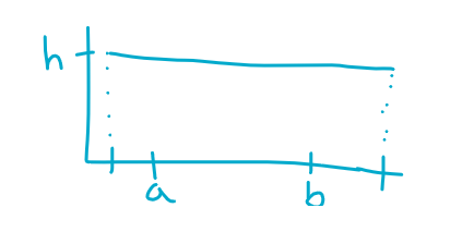
find proportion of values between a and b given a density curve (image on the left) (farthest left/right tick marks are the min and max bounds) (find h by doing A=base*height → 1=(max bound-min bound)(h) → solve)

• proportion = Area 

• Area = base*height = (b-a)(h) !!