Stats Spring Exam 1

EFA is based on…

the common factor model where variance is observed because of 3 sources.

Common Variance

Variance that’ influences multiple variables (latent factor)

Specific Variance

Variance specific to that variable

Communality

how much that factor accounts for the item. the proportion of variance explained by the common factors. range from 0-1 in orthogonal rotations. square of factor loadings in orthagonal rotations. having a uniform pattern

Uniqueness

how much the factors do not account for the item. 1- communalities. how much item doesn’t contribute to the factor structure

Complexity

How many factors are related to the item. extent to which observed variable (survey item) is influenced by multiple factors. Measures whether a variable is primarily associated with a single factor (low…) or spread across multiple factors (high…). Items that are high should be removed or revised. If value is close to or more than 2, remove or revise the item

What is the cutoff for secondary loadings in EFA?

.30

The value for complexity in EFA that indicates simplicity is..

1

The value for complexity in EFA that indicates complexity is..

more than 1. cutoff is 2.

Factor Loadings

how much the factor accounts for the item (similar to regression coefficient). Items with a higher factor loading are more accrutely measuring the factor. cutoff is .30

SS Loadings in EFA

eigen values after rotations. amount of variance accounted for by a factor after rotation

Proportion variance in EFA**

the proportion of total variance explained by each factor *after rotation). it’s the SS loadings / # of items. What % of the whole survey does this factor cover? so if it says 0.149, then PA1 accounts for 14.9% of the variance

Cumulative Variance in EFA

cumulative proportion of total variance explained by the factors after rotation. what % of the whole survey do all my factors cover?

Proportion Explained in EFA

proportion of common variance explained by each factor after rotation. what % of the shared signal does this factor cover?

Listwise Deletion

remove entire data cases (remove the entire person)

Pairwise Deletion

remove only the missing value and leave the rest of the person’s answer

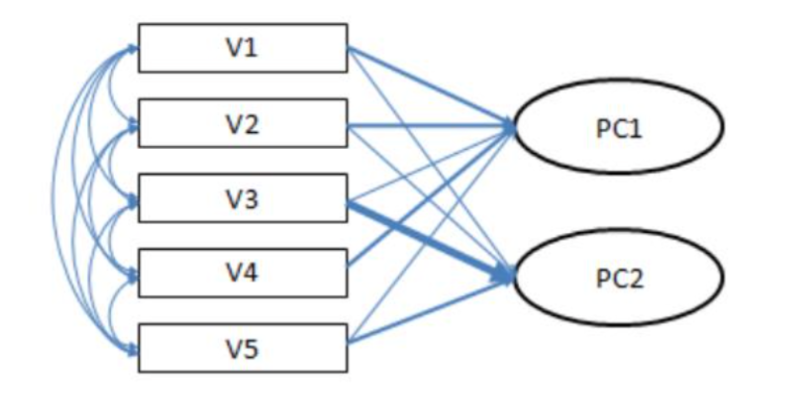
Principle Component Analysis (PCA)

type of exploratory factor analysis. transform the original variables into a new set of uncorrelated variables called Principle Components (combine items to create new components). focuses on variance maximization rather than explaining underlying latent structure. uses ALL variance and does not throw out unique variance. use when you have 500 variables and you just need ot squash them down into 10 variables so your computer can run regression faster. you don’t care what the 10 variables “mean” psychologically, you just need them to hold the data

Factor Analysis

goal is to find smaller number of interpretable factors to explain the correlations among a set of variables (items). basically correlation. used to study dimensionality of items

Dimensionality

number of underlying factors or constructs that explain the correlations between your observed variables

How is factor analysis different than cluster analysis?

Cluster analysis groups similar observations while factor analysis groups underlying variables

Exploratory Factor Analysis

a type of factor analysis. You use it to prove all these survey items probably are talking about one overarching thing. You check the correlations among items. you’re using it when you’re creating a test/survey. Basically, if you’re starting from scratch, you have to use this

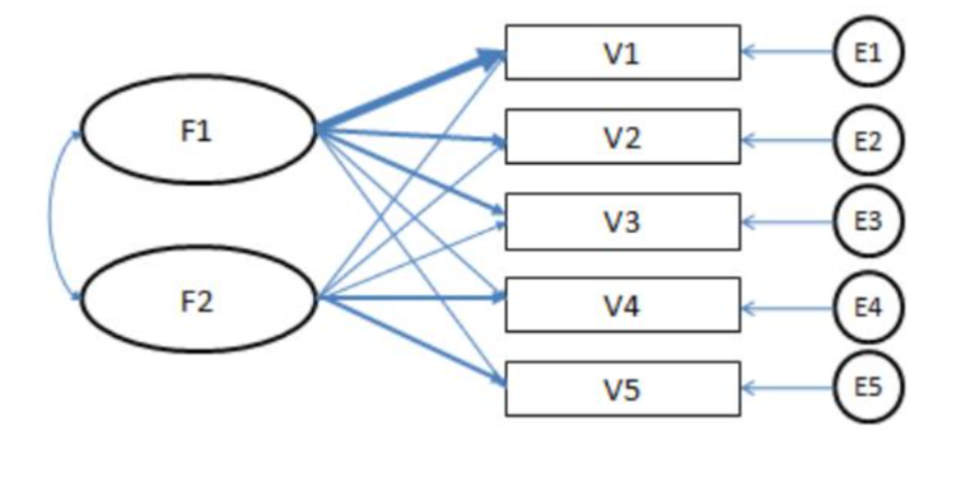
EFA

Observed Variance

common variance + unique variance

Unique variance

specific variance + measurement error

EFA Steps

1. Check KMO and Bartlett Test (assumption check)

2. Select extraction method

3. Check eigen values, scree plot, parallel anlaysis

4. Identify # of factors

5. Rotation

6. Interpretation: examine factor loadings, communalities, unqiueness, complexity

KMO Assumption check

tests if you have a big enough sample size for EFA. want it to be .50 or higher where the higher the better. general sample size recommended is 100-300

Bartlett Test assumption check

check in EFA if there’s a correlation among items. you want this to be significant

step 2 of EFA

Factor Extraction

Factor Extraction in EFA

You have determined in EFA that you have a large enough sample size and there is a correlation among items. but the correlation could be because of unique and common variance. we only care about common variance so you need to extract common factors first so you can ignore unique variance. you can use principal axis factoring or maximum likelihood

Principal Axis Factoring

most common extraction method for EFA

Eigen Values

indicate how much common variance that factor is responsible for

Which factor extraction method is most recommended?

Cattell Scree test. check the steepness of the line in the scree plot like the elbow method. Pick the steepest line and choose the factor in taht line that has the highest eigen value

Why do we need to rotate factors in EFA?

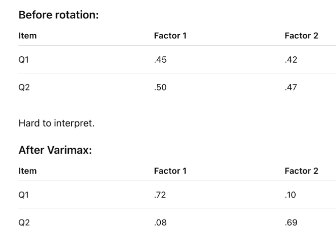
When factors are first extracted, the computer is greedy. It makes the first factor as large as possible, explaining as much variance as it can. This causes a factor matrix where every item correlates onto factor 1, making it impossible to tell what each factor actually represents. Before rotation, the axis are misaligned with these grouping where items tend to load moderately on multiple factors making the factor loading difficult to interpret. We rotate so that each item loads strongly onto only one factor (simple structure)

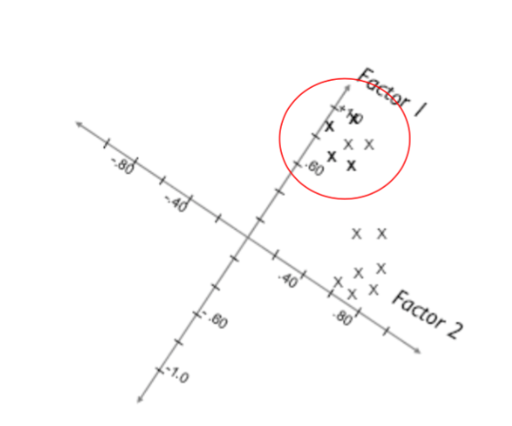
Orthogonal Rotation

factors are kept at 90 degree. You’re forcing the factors to be uncorrelated. Loadings range from -1 to 1 behaving like simple correlations. Most common is Varimax rotation which tries to maximize the variance of the squared loadings on each factor by producing high loadings on each factor and low loadings on each factor. Varimax rearranges teh factor axes after extraction so that each item loads highly on one factor and near zero on the other.

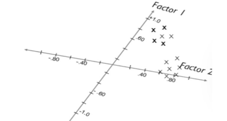
Oblique Rotation

in almost all cases, we use this rotation because it allows factors to be correlated and closer to reality in our field. items will now load strongly on one factor and cross-loadings are minimized. Factors are allowed to related to each other. Promax is the most popular. this rotation checks if there is a correlation between factors and items.

How to sort factor loadings?

higher correlation means items is more strongly tied with factor. aim for 5 or more items as the number of items shouldn’t be too few. strongly loaded items are around .5 to .9. the number of items in each factor shouldn’t be too many.

**Remove factor loadings less than .30.Negative values are just reverse coded. no need to check communality or uniqueness separately because they are tied to factor loadings.

You decide which factor the item belongs to based on the largest loading. if an item loads more than .30 on multiple factors, it’s cross-loading

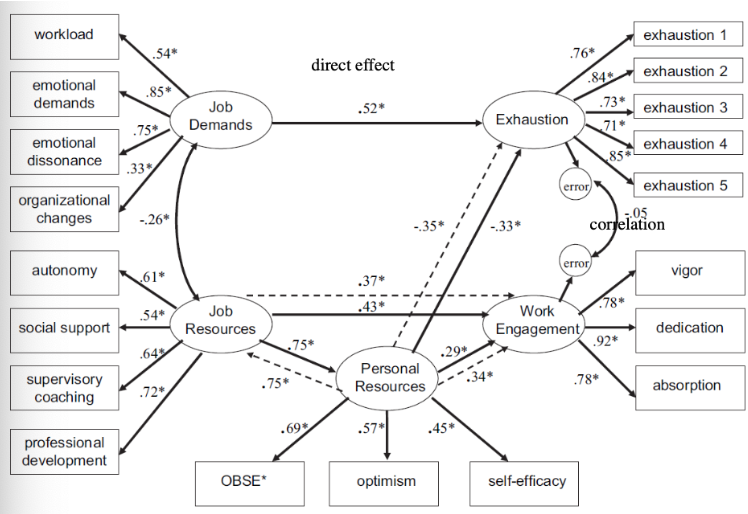
SEM (structural equation modeling)

combines measurement and structure. handles latent constructs by using multiple observed indicators. combines CFA and Path analysis where observed variables lead to latent variables and latent variables can directly affect each other

The latent variable “Job Demands” is assessed by 4 observed variables (assessed by means it’s the overarching thing)

Path Analysis

examines relationship among observed variables. NO latent variables. all are observable variables with tons of direct effects (a causes b). it’s a series of multiple regressions used to see how one variables leads to another in a chain.

---

→

Regression symbol (cause and effect)

Endogenous Variables

Dependent variables

Exogenous Variables

Independent variables

• Work Satisfaction (DV) depends on Job grade (IV)

  • Work Satisfaction ~ Job Grade

  • Make sure DV is on the left

• Workgroup Cohesion (DV) depends on Work Satisfaction (IV)

  • Workgroup Cohesion ~ Work Satisfaction

• In this example, work satisfaction is a DV and an IV

• Work Satisfaction correlates with Supervisor Satisfaction

  • Work Satisfaction ~~ Supervisor Satisfaction

• Endogenous Variables (DV): WS, SS, CS, SH, WC, OC, PW, PH

• Exogenous Variables (IV): JG, OT, JG-C

Confirmatory Factor Analysis

it’s a measurement model (it’s an SEM model). used for theory testing, check and confirms theory when there are clear hypotheses. Examines dimensionality and internal structure validity. used to detect construct bias and differential item functioning. used to evaluate convergent / discriminant validity using a multi-trait multi-method matrices

McDonald’s Omega

Estimating reliability. EFA and CFA used for estimated internal consistency. can use Cronbach’s alpha too

Differential Item Functioning

Items working differently across sub-groups (life is a party works well in US but not in other countries)

Does CFA look at causal relationships?

No, instead it tests if your survey questions load onto the concept you think they do. the observed variable is what causes the person to answer that. CFA includes latent variables and they can correlate but no direct effect between latent variables because it’s assuming items are only assessing one thing. Each latent variable has to have a minimum of 3 observed variables.

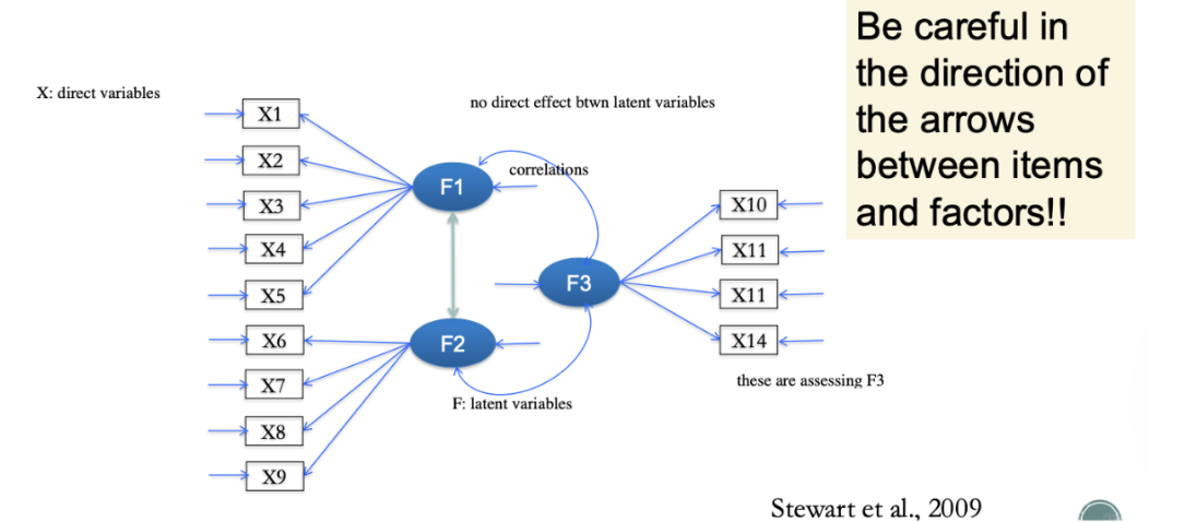
CFA

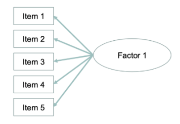
More CFA

The arrows are pointing away from the factor because we are measuring how much of that question’s variance is accounted for by the concept. The latent variable is the IV (circle) because it’s causing the item answers. Observed variables (the squares) are the DVs.

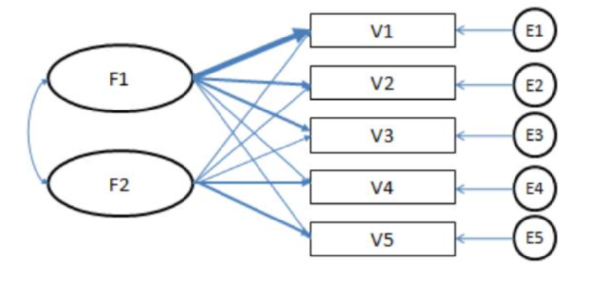
Difference between EFA and CFA diagrams

EFA, the latent variables (circles) are on the left pointing to EVERY observed variables (square) whereas in CFA, the latent variables are in the middle pointing to only designated observed variables

Common Variance: unlike in EFA where every item is mathematically linked to every factor, CFA strictly assumes that an item has 0 correlation with any factors other than the one it was specifically designed to measure

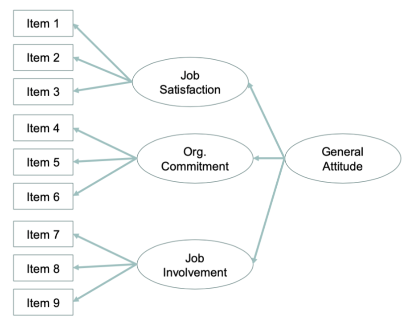
CFA example

• If the arrow points toward job involvement, it’d be PCA

• Job Satisfaction includes the variance of General Attitude

• Job Satisfaction consists of General Attitude Variance AND specific variance

• General Attitude is the IV, JS/OC/JI are IV and DP, Items are DP

• Jobs Satisfaction = a*General Attitude Variance + error

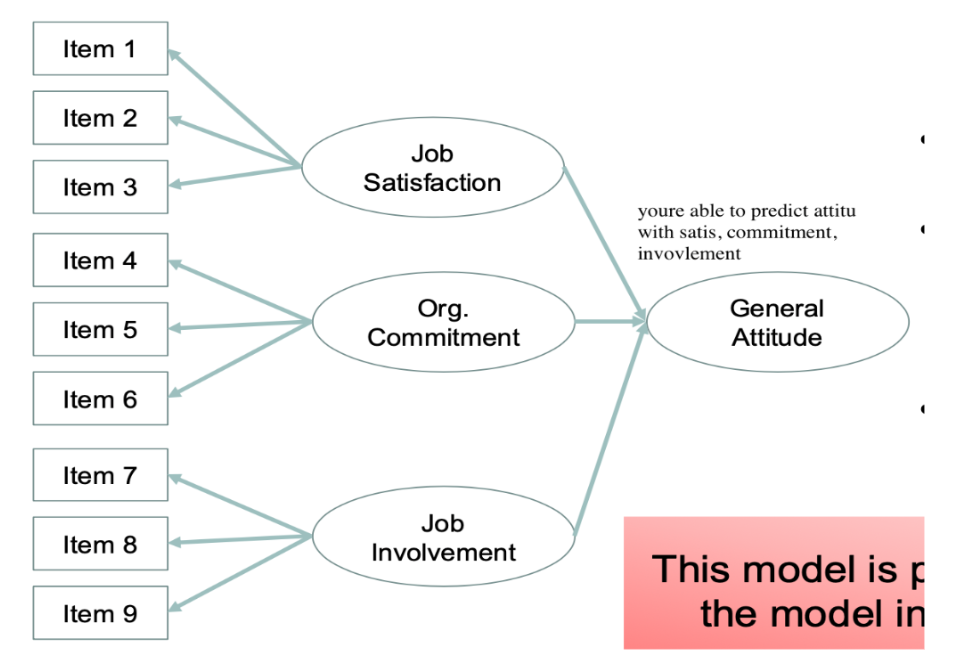
• Different than the previous model

• JS/OC/JI are purely IVs

• General Attitude is a DP (attitude is predicted by satisfaction, commitment, and involvement)

• GA = a*JS + b*OC + c*JI + error

• a,b,c are the Path Coefficients (the weights). They tell you how much each specific concept (like Job Satisfaction) contributes to the "General Attitude"

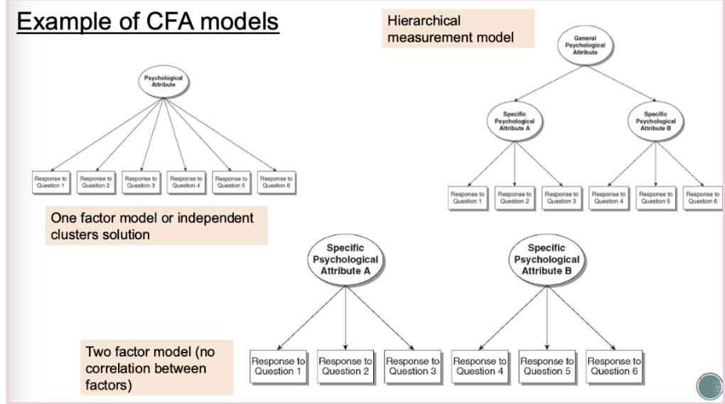
Difference between EFA and CFA

EFA: Every observed variable is allowed to link to every latent factor. The computer determines the "loadings" based on correlations. CFA; You constrain the model. You tell the software exactly which squares link to which circles. You "fix" the other paths to zero (meaning you assume there is no relationship). Because of, the factor loading cutoff limits are different,  EFA factor loadings are .3 but CFA is higher (.5). cut off point bc of calculation where it assumes the item is just assessing this factor. Assumption increases factor loadings.

CFA Steps

1. Collect data (want sample to be 300 or more)

2. Specify measurement model

3. Submit data to analysis

4. Check fit indices and parameter estimates

5. Modify model and re run if necessary

Step 2 of CFA: specify measurement model

1. You need to have the # of factors

2. Which items load onto which factors

3. Whether factors are orthogonal (90 degree) or potentially correlated (if more than 1 factor in the model)

4. - 3 INDICATOR RULE

   1. MUST BE AT LEAST 3 OBSERVED VARIABLES (ITEMS) FOR ONE FACTOR 

   2. Each observed variable must LOAD ONTO ONLY FACTOR (because CFA is an already established model that is supposed to have separate latent variables)

   3. ERROR OF THE ITEMS MUST BE MUTUALLY UNCORRELATED (If the errors of Item 1 and Item 2 are correlated, it suggests there is another hidden influence connecting them that you haven't accounted for. The rule assumes that the only reason the items are related is because of the main factor.)

   4. This model is theoretical so it can be broken but rare

   5. Be cautionary when adding error correlations.. In software like AMOS or Mplus, there is a tool called Modification Indices (MI). It effectively tells you: "Hey, if you correlate the error between Item 3 and Item 7, your model fit scores (like CFI or RMSEA) will look much better!" The Trap:

      • Statistical Merit: The model "fits" the data better.

      • Theoretical Failure: You might be correlating errors between two items that have absolutely no logical reason to be linked. This is called "overfitting." You are essentially forcing the model to match the quirks of your specific sample rather than representing a universal truth.

Step 3 of CFA

1. Actual data used to estimate parameters of the measurement model as specified by you

   1. Statistical software processes your raw data to calculate the numerical "weights" (loadings) and variances for the paths you defined in your theoretical model. This process converts your abstract diagram into a concrete mathematical representation of the relationships between your observed variables and latent factors.

   2. Evaluates how well the actual data “fit” with the measurement model in general

   3. This step uses statistical estimation to determine how closely your proposed theoretical structure aligns with the actual patterns in your collected data. By calculating fit indices, you can objectively verify whether your model accurately represents the real-world relationships between variables.

Step 4 CFA

1. Fit indices (how much the data fits to the model)

   1. Chi Square (x2): chi square is detecting if there is a difference between the theoretical model and the actual data. You don’t want a difference so YOU WANT THIS NON SIGNIFICANT SO P > .05. But it’s sensitive to sample size we don’t rely on this. Instead rely on RMSEA and CFI

   2. RMSEA: LESS THAN .06 SMALLER THE BETTER. a small RMSEA proves that your model is both accurate and concise. RMSEA tells us how much discrepancy exists between your theoretical model and the actual data, but it adjusts for the complexity of your model. A low RMSEA means your model explains the data efficiently without needing an excessive number of paths or correlations to "force" a fit. A high RMSEA means there is a lot of unexplained "leftover" error that your model failed to capture.Measures the amount of misfit per degrees of freedom.

   3. CFI: compares your model to a "null" model (where nothing is related). It tells you how much better your theory is than "nothing." WANT MORE THAN OR EQUAL TO .95 BIGGER THE BETTER. The higher the number, the more model is better than the null model

   4. SRMR: looks at difference in residuals between theoretical model and actual data. WANT LESS THAN .08 because the less difference in residuals means there’s less difference in the model and the data

   5. If good, check parameter estimates, aka factor loadings. If poor, examine modification indices to know how to improve the model

2. Check Parameter estimates aka the Factor Loadings

   1. you look at the specific "weights" or strengths of the relationships in your model

   2. Set a constraint: Because a "Factor" is latent (unobserved), it has no natural scale. The computer doesn't know if "Intelligence" should be measured from 1 to 10 or 100 to 1,000. To solve this, you must set a constraint to give the factor a scale. Usually set as 1 automatically in Jamovi

   3. Check Standardized estimates (std.all): WANT THE FACTOR LOADINGS (std.all) TO BE MORE THAN EQUAL TO .50. THEN YOU WANT IT TO BE SIGNIFICANT (p < .05)  Unstandardized Estimates: These are tied to the original units of your survey (e.g., a 1-5 Likert scale). They are hard to compare if different questions used different scales. Standardized Estimates: These usually range from -1.0 to +1.0. Think of these like correlation coefficients. A loading of 0.70 means the factor explains 49% (.70 squared) of that item’s variance. YOU WANT IT TO BE SIGNIFICANT SO LESS THAN .05 

3. Set a missing value method: When dealing with missing data in a CFA, you have to decide how the software should handle the "holes" in your dataset. If you don't choose a method, the software might default to something that biases your results.

   1. Full Information Maximum Likelihood (FIML): Gold Standard" for modern SEM and CFA. How it works: It doesn't actually "fill in" or create new data points (like imputation does). Instead, it uses all the available information from every participant to estimate the model parameters. If a person answered 9 out of 10 questions, FIML uses those 9 answers to help estimate the 10th based on how other similar people answered.Why it’s popular: It is highly efficient and produces unbiased results even if your data is "Missing at Random" (MAR). It allows you to keep your full sample size ($N$) instead of throwing people away.

   2. Exclude Cases Listwise (Listwise Deletion). Not recommended. How it works: If a participant skipped even one question in your entire survey, the software deletes their entire row. They are completely removed from the analysis. The Downside: * Power Loss: You lose a lot of data, which makes it harder to find significant results. Bias: If the people who skipped questions are different from the people who didn't (e.g., stressed people were too tired to finish the stress survey), your final "clean" sample no longer represents the real world.

4. Modification Indices: modify the indices if they weren’t good. Modify the items, take them out, etc

Step 5 CFA

1. When you have multiple models and are comparing them, check:

2. Compare the fit indices first to even know if the models are good in the first place (Chi Square is NOT significant bc if it was significant, it’d mean there was a big difference in the model and your actual data, RMSEA: less than .06 where smaller the better because it shows that your model is accurate and concise to the data, and CFI: more than  equal to .95 to show that compared to a null model, this model is really good)

3. Use AIC and BIC where SMALLER THE BETTER

= ~

Load on: means arrows point from factor to the items. So the items are loading onto the factor because the factor causes the items. Used in CFA and SEM

~

Regress on: causal path for calculation with correlation numbers. Only in SEM and path anlaysis because this is an entirely different meaning. When arrows point from the observed to observed, it’s talking about predicting, not what items are included in a latent variable. UNDERSTAND WE USE THIS WITH CORRELATION NUMBERS. IT’S TALKING ABOUT IV AND DV WHEREAS =~ IS TALKING ABOUT PUTTING WHY ITEMS ARE FROM A GROUP

~

Correlated with. Means there are correlations. CFA and SEM

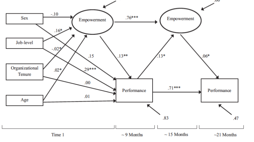
SEM example: Empowerment ~ Sex + Job Level + Org Tenure + Age (bc the arrows are pointing to the latent variable, it means it’s a regression, not a load on)

• Empowerment ~ Empowerment 

• Empowerment ~ Performance

• Endogenous Variables (DV): EM, Perf, EM, Perf

• Exogenous Variables (IV): Sex, Job level, Org tenure, Age

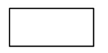
Observed variable

Latent variable: aren’t directly observed. inferred from other variables

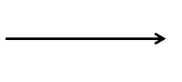
Direct effect (regression, cause and effect)

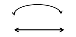
Correlation

Steps for Path Analysis and SEM

1. Collect Data (need sample size of 300 or more)

2. Specify the model

3. Submit data to analysis

4. Check fit indices and parameter estimates

5. Modify model and re-run if necessary

6. Interpret parameter estimates

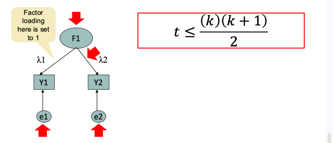
Underidentified Model

more estimated parameters (unknowns) than known information (data). can’t run model, can’t check indices, asking too many questions for the data you have. Example of an underidentified model: There’s only 2 items for the one latent variable, breaking the 3 indicator rule.

k (observed variables) = 2 

2 (2 +1) / 2 = 3

T (# of unknown parameter values) = 4 (variance of the latent variable, error variance of observed indicator 1, error variance of observed indicator 2, and factor loadings of one variable

4 is more than 3 (t is more than equation) so underidentified

Therefore formula is not establish and cannot estimate parameters

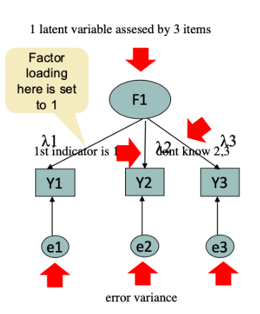
Just Identified Model

known info is equal to estimated parameters (just one answer). While the model can be estimated, it now can’t test model adequacy (fit indices don’t work because will always be “perfect” be definition). No leftever data to test if theory is actually true. Info = parameters. Can run it, can’t check indices because fit is perfect. Just enough data for one answer. RMSEA is automatically 0 and CFI is 1.

In Just-identified models, they can’t be found false: This isn't because your theory is brilliant; it’s because the math has been forced to account for every single correlation. You haven't tested a theory; you've just rewritten your data in a different "font.”

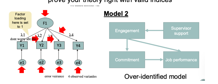
Overidentified Model

more known info than estimates parameters (unknown). Plenty of info. Necessary but not sufficient condition for identification. GOAL OF CFA AND SEM BC YOU HAVE EXTRA INFO so can calculate indices and determine if it matches the real world. More info than parameters. Can check indices bc have extra info. Extra data to prove your theory right with valid indices

To make it over-identified, increase the # of items/variables. Can estimate parameters and fit indices. Better than underidentified and just identified

We want to be over-identified because the goal of model testing is falsifiability. Always have “room for improvement” so we can test if our model is good or bad

Recursive Rule in SEM

Path analysis and SEM have to be … which means that they have to flow in one direction. In this way, the dependent variables can be ordered. We DON’T want non… as we don’t know the starting point

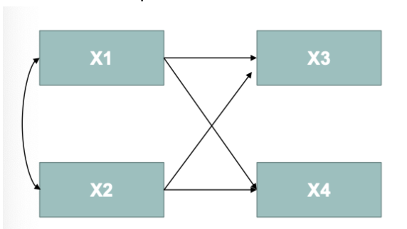
Recursive Model

X3 ~ X1 + X2 (X3 depends on X1 + X2)

X4 ~ X1 + X2 (X4 depends on X1 + X2)

X1 ~~ X2 (X1 and X2 are correlated)

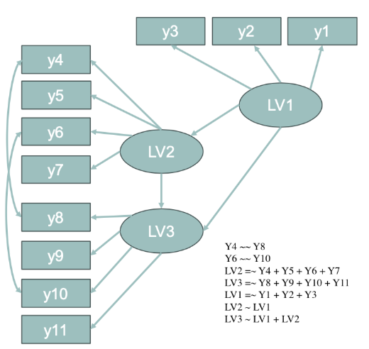
You only use regress on if the arrows are pointing from observed variables to the latent variables or latent variable to latent variable. This is because conceptually, if it was the other way around, it’d mean the observed variables are loading onto the latent variable. So it’s just the opposite. Then you can’t even load on latent variable to another latent variable so the only other option is regressed on.

Step 4 of SEM: Check fit indices and Parameter estimates

1. Fit Indices aka how well does the data “fit” the model

2. Chi Square (MORE THAN .05 SO NON SIGNIFICANT which indicates that there is not a big difference in your data and the model), RMSEA (LESS THAN .06, SMALLER THE BETTER, which means that your model is concise), SRMR (LESS THAN .08 -smaller the better- which means that there’s less left over variances between models), CFI (MORE THAN OR EQUAL TO .95 - higher the better - which means that your model is very good COMPARED TO A NULL MODEL)

3. Check if standardized estimates aka factor loadings (std.all) are more than .50 and significant (p less than .05.)  for the relations (ex: FB ~ PO:  std.all= .02 and 

4. If bad, examine the indices and modify model

Step 5 SEM: Modify the mdoel

1. Modification Index: an index showing how much model fit would improve if a fixed parameter were freely estimated.

CFA we don’t use mod indices bc we use it to check dimensionality of which item is good. SEM we use it to understand how to improve the model. use MODif indivex. provide info of which path you should use in model to get better fit indices. more exactly, application calculates how to improve chi squared test

1. "Hey, you currently have the path between Variable A and Variable B fixed at zero (meaning no arrow). If you 'freed' it (by adding an arrow) and let the data estimate the true value, your model's overall 'error' score (x2) would drop by the amount shown in the MI." When you look at your MI table, you are looking at a list of all the arrows you didn't draw. The software is testing every single possible missing arrow to see which one would help the most. As your notes say, just because the math says a window could go there doesn't mean it should. If you use it blindly, could lead to overfitting

2. MI shows how much your Chi Square will drop which you want because it means that there’s less difference between your data and the model (better fit). So usually a higher MI means a higher drop in Chi Square (and lower Chi square typ indicates better fit)

3. So the MI means the expected improvement in Chi Square if you add that path

   1. Ex: MI = 25. So chi square is expected to decrease 25 if path is added

4. WANT MI OF 3.84 AND HIGHER (adding MI of lower than 3.84 means adding the path doesn’t change the model)

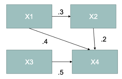
Step 6 SEM: interpret paramater estimates

1. Direct Effect: the pathway from the exogenous (IV) variable to the outcome (DV)

   1. X1 to X4 = .4

2. Indirect Effect: pathway from exogenous (IV) to the outcome (DV) through THE MEDIATOR

   1. X1 to X4: .3 * .2 = .06

3. Total Effect: direct effect + indirect effect

   1. X1 to X4 = .4 + .06 = .46

4. Standardized & Unstandardized: comparison is standardized. Prediction is unstandardized

   1. We use unstandardized to predict since it’s in the actual units. So one change in x leads to … in y

   2. We use standardized for comparison because it standardizes the units specifically for comparison. Like money and time is in the same unit now

You can modify the model by…

5. Remove paths: examine parameter estimates (CFI, RMSEA, CHI SQUARE), carefully handle it especially when removing non-significant paths. Removing paths just to improve model if is inappropriate bc of overfitting (model is good for the sample only, only now a description of the data and not a theory), doing so could inflate type 1 error (repeated path rimming = repeated testing) and increases false discovies. Non-significant doesn’t always mean there’s not a relationship (possible reasons could be because of suppression, multicollinearity, insufficient poiwer, part of an indirect effect. So path may still play a role in the model). Change confirmatory SEM into exploratory modeling (theory testing -> post hoc model fitting)

6. remove the non significant paths or items with low factor loadings (doesn’t appear in Path, only CFA and SEM), and try one by one because sometimes removing paths decrease fit indices

7. Add paths: examine modification indices (more than 3.84). Pick up a suggestion with largest MI. make sure don’t blindly add it.

Why is your SEM model broken?

1. In SEM, when your Chi-square is significant or your fit indices (CFI/RMSEA) are poor, it’s usually because the mathematical relationship between your survey questions (items) and your concepts (latent variables) is messy.

2. Insufficient Items (Quantity): If the items are insufficient measuring the latent variable. A latent variable (a concept you can't measure directly, like "Happiness") usually needs at least 3 items (questions) to be mathematically "identified." The Problem: If you only use 1 or 2 questions to define a concept, the computer doesn't have enough "information" to calculate the error vs. the true score. It's like trying to define a 3D object using only one photo; you're missing the depth. The Fix: Add more related questions to "triangulate" the concept. Consider adding more items but ensure they are theoretically appropriate.

3. Item Variance (Quality of Spread): Too Small: If everyone answers "5" on a 1–5 scale for a specific question, that item has no variance. If there is no movement in the data, the model can't see how that item relates to anything else. The math "stalls." Extremely Large: This usually happens if your scales are inconsistent (e.g., one question is 1–5, another is 0–1,000). The computer struggles to balance these huge differences, leading to "instability" (errors in the output). The Fix: Check for outliers or rescale your data so all items are on a similar playing field.

4. Correlated Errors (Hidden Relationships): The Logic: When you measure a concept, you assume the "errors" (the part of the question the model can't explain) are random. The Problem: Sometimes two questions are so similar (e.g., "I feel sad" and "I feel unhappy") that their errors are actually linked. The Modification Index (MI) will flag this and suggest you "correlate the errors." The Warning: Only do this if you can explain why they are linked. If you just click "add" on every suggestion to make your fit look better, you are "cherry-picking" results that won't hold up in a different study.

Endogenous Variable: OUTCOME/DEPENDENT VARIABLES: variable in model that’s changed or determined by its relationship with other variables in the model. 

Exogenous Variable: INDEPENDENT VARIABLE: determines endogenous. Never the dependent variable.

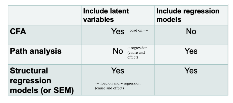
Differences between CFA, path and SEM

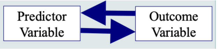
Reciprocal Causation

Two variables cause each other, “spiral effect”/ cyclical. Ex: marriage and happiness

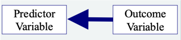
Reverse Causation

causal direction is opposite from what’s hypothesized. Ex: Married people are more likely to be happy. Reverse causation: happy people are more likely to attract people and be married

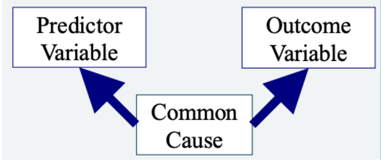
Common - Causal Variable

Some unknown third variables is actually influencing both the variables. “Spurious correlation”. Ex: ice cream sales and drowning rates are positively correlated. Third variable is summer.

Causal Claim Requirements

1. Covariance: two variables must covary (pos- move in same direction, neg- move in opp direction but both moving together)

2. Temporal Precedence: cause variable comes before the effect variable

3. Internal Validity: study eliminates alternative explanations

Regresion Models

General Linear Model

Generalized Linear Model

Generalized Linear Mixed Model

General Linear Model

• Linear Line

• Methods for data that is normally distributed

• T-test (compares the means of two groups to determine if they’re significantly different from one another, assumes the data in each group is normally distributed), ANOVA (Analysis of Variance: compares means of at least 3 groups, assumes residual errors are normally distributed), simple regression (relationship between DV and IV- continuous variables), multiple regression (relationship between DV and 2 or more IVs) (residuals are normally distributed)

• Predicts continuous numbers

Generalized Linear Model

• Methods for DV that are not normally distributed. Uses maximum likelihood to model nonlinear relationships like non-normal data (like binary)

• Logistic regression (used for binary classification, predicts probability of categorical outcome, etc)

Generalized Linear Mixed Model

• clustered data

• Clustered, hierarchical, or repeated measures data, allowing for random effects.

• Includes both fixed effects (general trends) and random effects (subject/group variation)

• Methods for nested data (hierarchical levels of grouped data like purchased items -> name, price, quantity)

• Hierarchical Linear Modeling (HLM- hierarchical data structures where lower-level units (Level 1) are nested within higher-level units (Level 2). 

• Level 1 (Individual): Analyzes relationships within groups (e.g., student ability on test scores).

• Level 2 (Group): Analyzes how group-level factors affect Level 1 relationships (e.g., school funding on test scores). Etc

Hierarchical Linear Modeling

an advanced regression model for nested data (the predictor variables are varying at hierarchical levels.) separate the effects of IVs by level in data analysis

• Hierarchical Levels are when the results vary depending on the levels (there's the whole data- higher level, and sub-groups - lower level). Typical analysis of hierarchical levels are Hierarchical Linear Modeling (analyzes data nested in groups (e.g., students in schools) by accounting for variance at multiple levels simultaneously. It works by creating nested regressions: Level 1 models individual relationships, while Level 2 models how group-level variables affect Level 1 intercepts and slopes) and Multilevel SEM (break down variance into a between cluster component representing group-level means and a within cluster component representing individual deviations from the group mean

  • Level 1 (Within): Models relationships between individuals within their groups (e.g., how student motivation relates to student achievement within a specific classroom).

  • Level 2 (Between): Models relationships between group-level aggregates (e.g., how average classroom motivation relates to average classroom achievement).

  • Simultaneous Estimation: MSEM estimates structural paths and latent factors at both levels at the same time using frameworks like the lavaan package in R.

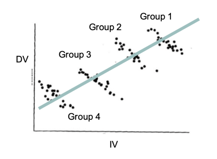
Nested Data

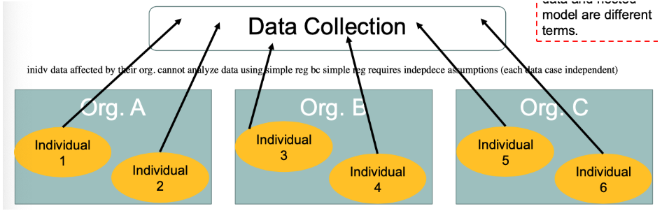
Nested Data: hierarchy where smaller units are tucked inside larger units

• Imagine you are measuring the productivity of individual employees (Level 1) who work within specific departments (Level 2). The data is naturally "nested" because employees are clustered within those departments.

• Ex: 1st level: job satisfaction, 2nd level: climate of department

• 1st level variable affected by 2nd level variable

• Ignoring nesting leads to inaccurate conclusions (e.g., assuming an employee's success is independent of their team leader). Multilevel modeling is required to properly analyze these structures and avoid pitfalls like the "atomistic fallacy," where higher-level organizational factors are wrongly ignored

• Data cases in a lower level are included in only one higher level group: this means: there is a "Mutually Exclusive" Rule: In a nested data structure, a "case" (the individual data point) cannot be a member of multiple groups at the same time. If it were, the data would be considered cross-classified rather than purely nested. 

  • Examples: Education: If you are studying students (Level 1) nested within classrooms (Level 2), the rule states that Student A can only be in Classroom 1. They cannot be half-enrolled in Classroom 1 and half-enrolled in Classroom 2 for the purposes of that specific analysis.

  • Corporate: If you are looking at employees nested within departments, an employee belongs strictly to "Marketing" or strictly to "Finance."

• The mutually exclusive rule is important because: If a case belonged to multiple groups, it would be impossible to cleanly calculate how much of the "error" or "variance" in the data is caused by the group versus the individual.

Nested Model

a relationship between two statistical models. This is a technique used to see if adding more variables actually makes a model better. Model A is "nested" within Model B if Model A is simply a restricted version of Model B. In other words, Model A contains a subset of the predictors found in Model B. when you are trying to decide if adding complexity to your research is actually worth it—nested models are used for comparison.

• Imagine you are a researcher trying to understand what makes people happy at work. You collect data on Salary and Autonomy (how much freedom they have).

  • Model 1: The Simple Model (Reduced): you believe that money is the only thing that matters.

    • Equation: Job Satisfaction = B0 + B1(Salary)

    • Status: This is the "Nested" model because it is a subset of the next one

  • Model 2: The Complex Model (Full): add Autonomy to the equation to see if it explains more of the "why" behind satisfaction.

    • Equation: Job Satisfaction = B0 + B1(Salary) + B1(Autonomy)

    • Status: This is the "Parent" model.

  • Why these are "Nested": Model 1 is nested within Model 2 because Model 1 is just Model 2 with $\beta_2$ forced to be zero. You haven't changed the math or the data; you’ve just "constrained" or removed one piece of it.

  • How you use them in the real world: Researchers use a Likelihood Ratio Test or a Chi-Square Difference Test to compare these If the difference is significant: It means Autonomy adds "unique value." You should keep the more complex model and If the difference is NOT significant: It means Autonomy doesn't really add anything new that Salary wasn't already covering. In the interest of parsimony (keeping it simple), you would stick with Model 1.

• Whenever collecting data from multiple organizations, you cannot just use simple regression as the people within each organization are no longer independent of each other. The organization is what affects them. Therefore why must use Hierarchical Linear Modeling. This scenario describes the violation of independence of observations assumption which requires that one person’s score has absolutely no relationship with another person’s score (which is automatically broken in nested data where people’s scores are assumed to be related within an organization). If you ignore the nesting and run a standard regression, your standard errors will likely be too small. This makes your results look more "statistically significant" than they actually are, leading to Type I Errors (finding an effect that isn't really there).

Mediation Analysis