Booklet 8 - Aggregate Expenditure

Define AE

Sum of all expenditure on final goods & services undertaken in the economy during a specific time period

AE Formula

C + Ip + G + (X-M)

doesn’t include inventories

Define GDP

Final value of all goods & services produced in a country during a year

GDP Formula

C + Ia + G + (X-M)

includes inventories

Differentiate between AE & GDP

The value of inventories (unsold stock) is included as part of actual investment when calculating GDP whereas it is not included in planned investment when calculating AE.

What do you discuss when asked about the Categories of Consumption:

Expenditure on Non-Durable Goods

Expenditure on Durable Goods

Expenditure on Services

Category of Consumption - Expenditure on Non-Durable Goods

Consumed shortly after purchase (within three years), including perishables such as food, drink &packaged products, clothing &footwear. Regarded as essential or non-discretionary, as it satisfies regular needs. This portion of consumption is fairly stable over time – typically counting for about 35 per cent of total consumption expenditure

Category of Consumption - Expenditure on Durable Goods

Last three or more years - including major appliances (washing machines, fridges), small appliances goods (kettle, toasters, microwaves), sporting equipment & motor vehicles. Spending is usually discretionary & can be postponed or brought forwards depending on the individual household’s circumstances. Discretionary spending is money spent by consumers on goods & services other than necessities such as food & fuel. Expenditure on durable goods accounts for approximately 15 per cent of consumption spending.

Category of Consumption - Expenditure on Services:

Intangible, usually provide transitory satisfaction of wants - items such as education, transport, health, &recreation. Spending on services makes up the largest part of consumption, accounting for approximately 50 per cent of all household expenditure. Some services are regarded as essential, such as health services & transport, while others are discretionary such as entertainment & leisure.

What do you Discuss when asked about Factors Affecting Consumption:

Identify what proportion of AE Consumption is - 52%
Level of Disposable Income (Yd)

• Increase in Consumption/AE

• Decrease in Consumption/AE

Interest Rates (Cost of Credit)

• Increase in Consumption/AE

• Decrease in Consumption/AE

Government Policy

• Monetary Policy

• Fiscal Policy

• Increase in Consumption/AE

• Decrease in Consumption/AE

Consumer Expectations:

• Increase in Consumption/AE

• Decrease in Consumption/AE

Asset Prices (Household Wealth)

• Increases in Consumption/AE

• Decreases in Consumption/AE

Other Demographics:

• Increase in Consumption/AE

• Decrease in Consumption/AE

Factors Affecting Consumption - Level of Disposable Income:

The level of disposable income—household income after taxes—is a key determinant of consumption. Higher disposable income increases households’ ability to spend, leading to greater consumption and higher aggregate expenditure. Conversely, lower disposable income reduces spending capacity, decreasing consumption and aggregate demand. Thus, consumption rises and falls in direct proportion to changes in disposable income.

Factors Affecting Consumption - Interest Rates (Cost of Credit)

Interest rates, as the cost of borrowing and return on saving, significantly affect household consumption. Low interest rates reduce borrowing costs and make saving less attractive, increasing disposable income available for spending and boosting aggregate consumption. Conversely, high interest rates increase borrowing costs and encourage saving, reducing disposable income for consumption and lowering aggregate expenditure. Thus, consumption is inversely related to interest rates.

Factors Affecting Consumption - Government Policy

Government policy affects household consumption through monetary and fiscal measures.

• Monetary policy: Higher interest rates (contractionary policy) increase borrowing costs, reducing households’ disposable income and spending power, which lowers consumption and aggregate expenditure.

• Fiscal policy: Contractionary fiscal measures, such as higher taxes or reduced government spending, reduce household income, decreasing consumption and aggregate expenditure.

Factors Affecting Consumption - Consumer Expectations:

Consumer expectations influence consumption by shaping households’ confidence in the economy. When consumers anticipate economic growth, rising incomes, or stable prices, they are more likely to increase spending on goods and services, boosting aggregate expenditure. Conversely, negative expectations—such as fears of unemployment, inflation, or declining asset values—can lead households to cut back on spending and increase saving, reducing consumption and aggregate demand.

Factors Affecting Consumption - Asset Prices (Household Wealth)

Asset prices affect consumption by influencing household wealth and confidence. When the value of financial assets (e.g., shares, superannuation) or real assets (e.g., property, vehicles) rises, households feel wealthier, increasing their willingness to spend. This boosts aggregate consumption and expenditure. Conversely, falling asset prices reduce perceived wealth, lowering consumption and aggregate demand.

Factors Affecting  - Other Demographics:

Demographics affect consumption by influencing the total number of consumers in the economy. An increase in population raises demand for goods and services, boosting aggregate consumption and expenditure. Changes in population size, age distribution, or household composition can also alter consumption patterns, shaping overall economic activity.

What do you discuss when asked about Categories of Investment:

Identify what proportion of AE Investment is - 19%

Define Business Investment

Define Housing Investment

Define Business Spending:

Privately funded business spending on capital goods used in production - including equipment, machinery & buildings.

Define Housing Investment

Private expenditure on new housing & apartments

What do you discuss when asked about Factors Affecting Investment

Interest Rates (Cost of Credit)

Level of Past Profits

Business Expectations

Government Policies

Factor Affecting Investment - Interest Rates (Cost of Credit)

Interest rates strongly influence business investment decisions because they determine the cost of borrowing. Higher interest rates increase borrowing costs, discouraging firms from investing in new capital, which reduces investment expenditure and aggregate demand. Conversely, lower interest rates make borrowing cheaper, encouraging investment, expanding capital expenditure, and increasing aggregate expenditure. Real interest rates, which account for inflation, are particularly important as they reflect the true cost of credit.

Factor Affecting Investment - Level of Past Profits:

The level of past profits affects investment because retained earnings provide firms with internal funds to finance new capital projects. When profits are high, businesses have more resources to invest in new equipment, facilities, or technology, boosting investment expenditure and aggregate demand. Conversely, during periods of low profits, firms may delay or reduce investment, lowering capital spending and aggregate expenditure.

Factor Affecting Investment - Business Expectations:

Business expectations affect investment because firms’ confidence about future economic conditions shapes their willingness to invest. Positive expectations about future sales and profits encourage firms to increase planned investment in capital, boosting aggregate expenditure. Conversely, negative expectations or uncertainty about the economy can lead firms to delay or reduce investment, lowering aggregate expenditure.

Factor Affecting Investment - Government Policies:

Government policies influence investment through monetary and fiscal measures.

• Monetary policy: Higher interest rates (contractionary policy) increase the cost of borrowing, discouraging businesses from taking loans to invest in capital, reducing investment expenditure and aggregate demand.

• Fiscal policy: Contractionary fiscal measures, such as higher company taxes or reduced government spending, lower firms’ retained earnings and profits available for investment, decreasing investment expenditure and aggregate demand.

What do you Discuss when asked about Categories of Government Spending:

Current Spending G1

Capital Spending G2

Current Spending G1

Expenditure on the day-to-day business of government in its core functions like health, education, social welfare and defence. This includes wages and salaries and the purchasing of goods and service

Capital Spending G2

Spending on productive machinery and public infrastructure such as power and water supply, roads, railways and communication networks

What do you Discuss when asked about Factors Affecting Government Spending:

Discretionary Changes (Optional Changes)

Automatic Changes (Forced Changes)

Stabilising Macroeconomic Fluctuations (Economic Obligations)

Factors Affecting Government Spending - Discretionary Changes (Optional Changes)

Governments will increase and decrease spending in accordance with government policy objectives such as social policies, infrastructure, health and education. For example, the Federal Government is contributing $1.7b to Perth’s Metronet project (G2). This increases government spending and therefore increases aggregate expenditure.

Factors Affecting Government Spending - Automatic Changes (Forced Changes)

Automatic changes in spending will occur depending on the phase of the business cycle. In a contractionary phase, there will be more unemployment and therefore government spending on welfare will increase. For example, during the Covid pandemic, government spending on welfare payments such as JobSeeker (G1) increased therefore increasing aggregate expenditure.

Factors Affecting Government Spending - Stabilising Macroeconomic Fluctuations (Economic Obligations)

In a contractionary phase, governments may actively increase spending in an attempt to increase economic activity. For example, during the pandemic, increases in Jobkeeper (subsidy) and Jobseeker (transfer payment), caused government spending (G1) to increase therefore increasing aggregate expenditure

What do you Discuss when asked about Categories of Net Exports (X-M)

Identify Net-Exports as a proportion of AE - 3%.

Define Exports

Define Imports

Define Exports

Foreign purchases of goods and services produced in Australia are exports and add to aggregate expenditure

Define Imports

When Australians purchase goods and services from overseas and reduce aggregate expenditure

What do you discuss when asked about Factors Affecting Net Exports

Level of Economic Activity

Exchange Rates

Terms of Trade

Presence of Trade Barriers

Level of Economic Activity as a Factor Affecting Net Exports

The level of economic activity both domestically and overseas plays a crucial role in determining net exports:

• Domestic activity: When Australia’s GDP grows strongly, households and businesses increase their demand for goods and services. Since Australia has a relatively small manufacturing sector, much of this demand is met through imports (e.g., manufactured goods, machinery, technology). As imports rise, net exports fall, reducing aggregate expenditure.

• Overseas activity: When major trading partners (such as China, Japan, or the US) experience strong economic growth, their higher employment and income levels drive up demand for imports, including Australia’s exports (e.g., minerals, agricultural goods, education, and tourism). This boosts Australian exports, increasing net exports and aggregate expenditure.

Exchange Rates as a Factor Affecting Net Exports

Exchange rates directly affect the relative price of imports and exports, and therefore net exports:

• Appreciation of the AUD: When the Australian dollar strengthens, it increases the purchasing power of Australian consumers and businesses. Imports become cheaper in AUD terms, leading to an increase in imports. At the same time, Australian exports become relatively more expensive for foreign buyers, reducing the competitiveness of non-commodity exports (such as education, tourism, and manufactured goods). Both effects decrease net exports, lowering aggregate expenditure.

• Depreciation of the AUD: When the dollar weakens, imports become more expensive, discouraging import consumption. At the same time, Australian exports become relatively cheaper on world markets, making them more competitive. Export volumes increase, improving net exports and boosting aggregate expenditure.

Terms of Trade as a Factor Affecting Net Exports

Movements in the terms of trade (ToT) – the ratio of export prices (XPI) to import prices (MPI) – strongly affect Australia’s net exports, since they determine how much can be imported for a given level of export revenue:

• Increase in ToT: When export prices rise relative to import prices, Australian exporters (e.g., mining and agriculture) receive higher income for the same volume of exports. This lifts national income and aggregate demand through increased export earnings. At the same time, lower relative import prices mean Australia can import more for less, often reducing the overall value of imports. Together, this improves the trade balance, increases net exports (NX), and raises aggregate expenditure (AE).

• Decrease in ToT: When export prices fall relative to import prices, exporters earn less income, reducing export revenue and lowering national income. Meanwhile, relatively more expensive imports may worsen the trade balance if import volumes remain steady. This reduces NX and therefore contracts AE.

Presence of Trade Barriers as a Factor Affecting Net Exports

tariffs, quotas, subsidies, or other restrictions—directly impacts Australia’s net exports by influencing both the demand for exports and the supply of imports:

• Barriers on Australian exports (imposed by trading partners): If countries place tariffs or quotas on Australian goods (e.g., agricultural or manufactured products), the price of these goods rises in foreign markets, making them less competitive. This reduces demand for Australian exports, lowering export revenue, decreasing net exports (NX), and contracting aggregate expenditure (AE).

• Barriers on imports into Australia (imposed by Australia): Protectionist measures like tariffs on imports may reduce the volume of imports purchased by Australian consumers and businesses. This could, in the short term, improve NX since imports fall. However, this often provokes retaliation from trading partners, who may impose counter-tariffs on Australian exports, ultimately reducing export volumes and worsening NX.

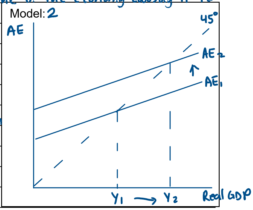
Using the AE Model to show an Increase in a Component of AE (Positive Multiplier)

As seen in model 2, an increase in one of the components of AE causes an upward shift of the AE curve from AE1 to AE2. This impacts the real level of output & income in the economy causing it to increase from Y1 to Y2. This leads to the positive multiplier effect as the increase in AE which is the vertical distance between AE1 & AE2 creates a larger increase in output & income which is the horizontal difference between y1 & y2. An increase in AE is associated with an economic upturn in the business cycle as seen in Model 1 (business cycle model).

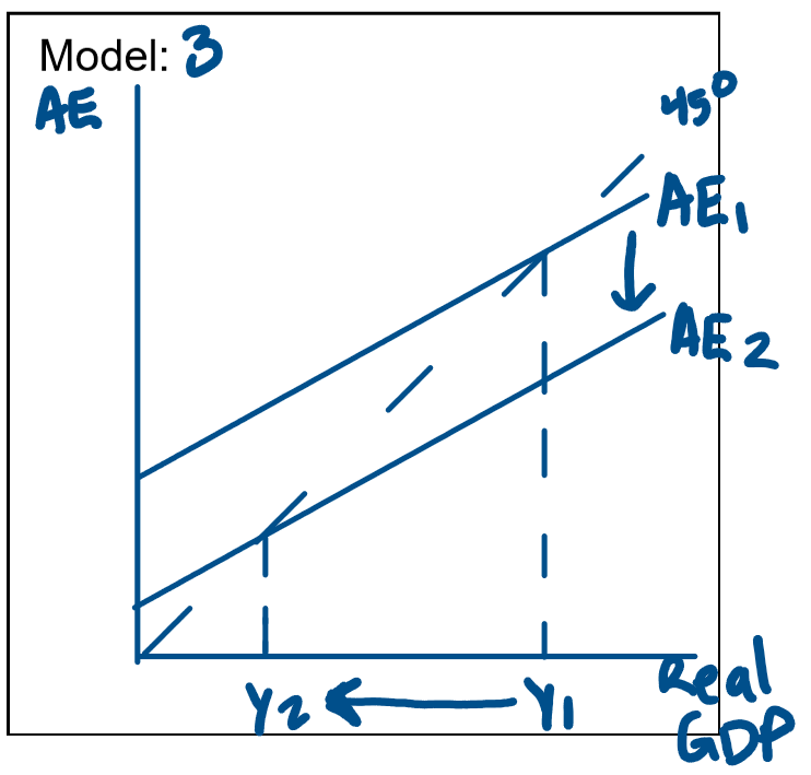
Using the AE Model to show a Decrease in a Component of AE (Negative Multiplier)

As seen in model 3 a reduction in one of the components of AE causes a downward shift of the AE curve from AE1 to AE2. This impacts the real level of output and income in the economy, causing it to fall from Y1 to Y2. This leads to the negative multiplier because the decrease in AE which is the vertical distance between AE1 to AE2 creates a larger decrease in output and income which is the horizontal distance between Y1 and Y2. A reduction in AE is associated with an economic downturn in the business cycle as seen in model 1.

What do you Discuss when Asked about the Relationship between Income, Consumption & Savings:

Consumption Function

• Formula

Average Propensity to Consume

• Formula

Average Propensity to Save

• Formula

Consumption Function & Formula

Describe the relationship between income (Y) & what is spent on Consumption (C)

Yd = C + S

Average Propensity to Consume & Formula

Proportion of total income spent on consumption

APC = Consumption (C) / Income (Y)

Average Propensity to Save & Formula

Proportion of total income that is saved

APS = Savings (S) / Income (y)

What do you discuss when asked about the Consumption Function:

Consumption Function Formula

Autonomous Consumption

Induced Consumption/Marginal Propensity to Consume

• Formula

If given data:

• Draw a diagram

• State the relative consumption function

Assumptions for the MPC & MPS

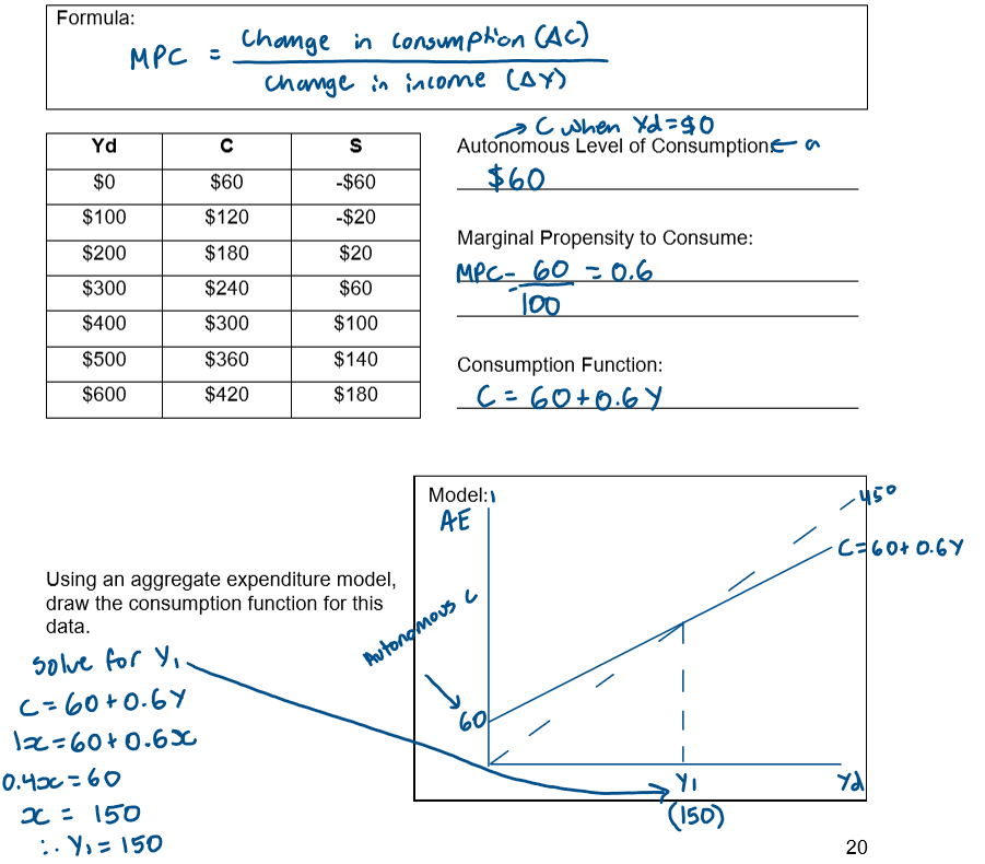
Define Autonomous Consumption

Part of consumption which occurs even when income is zero. This is the minimum quantity of goods to survive. It is constant and does not vary with income. It is the vertical intercept- the point where the consumption function meets the y-axi

Define Induced Consumption/Marginal Propensity to Consume

Part of consumption which occurs because income increases. Another name for b is the Marginal Propensity to Consume (MPC). MPC is the fraction of an increase in income spent on consumption.

Induced Consumption/Marginal Propensity to Consume Formula

Change in Consumption / Change in Income

Example of a Consumption Function Model & Question

Effect of an increase in Autonomous Consumption on the Consumption Function:

Increase in Consumption shifts curve up from C1 to C2

Effect of a Decrease in Autonomous Consumption on the Consumption Function:

Decrease in Autonomous Consumption shifts curve down from C1 to C2

Effect of an Increase in the MPC on the Consumption Function

Increases the consumption function from C1 to C2, but remains at the same value along the y-intercept

Effect of a Decrease in the MPC on the Consumption Function

Decreases the consumption function from C1 to C2, but remains at the same value along the y-intercept.

What do you discuss when asked about the Savings Function:

Savings Function Formula

Define Savings

Define Marginal Propensity to Save (MPS)

• MPS Formula

Break Even Point

Savings Function Formula:

S = D + (MPC x Y)

Define Dis-Savings

Savings when Yd = $0

When savings is negative this is defined as dis-savings

Define Marginal Propensity to Save (MPS)

The fraction of income not spent on consumption, it is the slope of the savings function.

MPS Formula

MPS = Change in Savings / Change in Income

Define the Breakeven Point

When the level of savings changes from negative to positive

The Full Aggregate Expenditure Function

Define Consumption

Define Investment (Ip)

Define Government Spending

Define Exports

Define Imports

Define Consumption - AE

Both an autonomous level & induced component.

Autonomous consumption is the minimum amount of consumption necessary for economic participants to survive

Induced consumption depends on income & is determined by the MPC

Define Investment Ip - AE

Assumed to be independent of the level of GDP & therefore considered autonomous, this assumes factors affecting both discretionary & automatic spending are constant.

Define Government Spending - AE

Independent of the level of GDP & therefore considered autonomous.

Define Exports - AE

independent of the level of income & therefore autonomous

Define Imports - AE

Autonomous level of imports & and induced component dependent on income (GDP) 

Induced imports increase with GDP

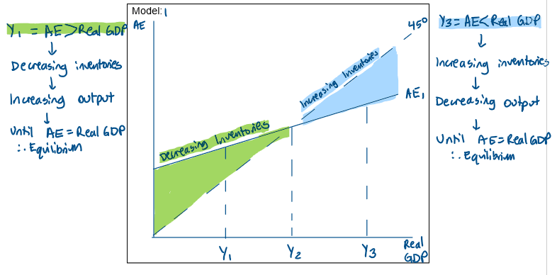
Concept of Macroeconomic Equilibrium Including the Role of Inventories:

At Y1, AE is greater than real GDP, leading to a decrease in inventories as firms sell more than they produce. The reduction in inventory levels signals firms to increase their production, firms hire more labour thereby increasing employment. This increase in production & employment leads to a rise in real GDP. However as real GDP rises, the increase in AE slows due to the slope of the AE curve reflecting the MPC. The economy continues to adjust unit it reaches a new macroeconomic equilibrium at Y2, where AE equals real GDP & income levels are stable.

At Y3, Real GDP exceeds AE resulting in increasing inventories as firms produce more than what is being consumed. The accumulation of inventories signals firms to decrease thier production to prevent excess unsold goods. As firms reduce production, they demand less labour, leading to a decrease in employment. This reduction in production & employment causes a decline in real GDP. As real GDP falls, the decrease in AE occurs at a reduced pace due to the slope of the AE curve which moderates the decline & reflects the MPC. The economy adjusts until it reaches a new macroeconomic equilibrium at Y2, where AE equals real GDP & income levels are stable.

Multiplier Formula

K = 1 / MPS

or

K = 1 / 1 - MPC

Change in Income Formula

y = K x change in autonomous spending

Characteristics of the Multiplier

• he multiplier takes time to work. The effect is not immediate. The rounds of spending and spending take months or years.

• The multiplier works in both directions.

• A rise in the level of autonomous investment results in an even larger increase in the level of income.

  • Examples:
    Construction of Perth’s Metronet (public transport/train system) estimated at $11.5 billion ($1.7 billion by the Federal Government in 2024/25) o Construction of Melbourne’s North East Link (highway/road network) estimated at $26.1 billion ($3.3 billion by the Federal Government in 2024/25)

• A reduction in the level of autonomous investment means a larger decrease in the level of income (the multiplier in reverse). Examples: Covid 19 recession, large decrease in investment due to uncertainty.

• The size of the MPC and the multiplier are directly related. The higher the MPC, the higher the value of the multiplier.

The Size of the Multiplier:

Size of the economy’s MPC determines the size of the multiplier

The higher the MP the greater the final value of additional income 

the higher the value of the MPS the lower the final value of additional income

Using an AE model demonstrate & explain the Multiplier Effect when there is an increase in investment on the Australian economy:

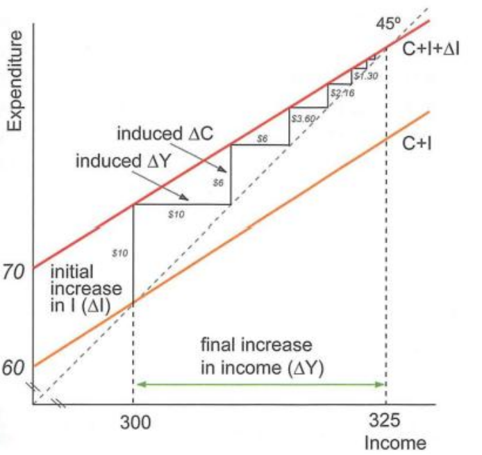
The multiplier shows how an increase in planned injections into the economy leads to a larger increase in output and income. This is because the initial injection sets off rounds of spending. It is based on the idea that ‘one man’s spending is another man’s income’.

In the first round investment, a new income of $10b is generated for workers to either spend or save their income. Assume in a mining venture, workers such as engineers and construction workers are employed and paid for their labour. As MPC is 0.6, workers spend $6b on goods and services and save $4b.

In the second round, as $6b is spent by the first group of people. This will flow into other groups of the economy and they will receive $6b as their income. Assume the workers in the mining site venture out to buy food from Woolworths. The employees at Woolworths will receive a new income of $6b. These second group of employees will spend 60% of $6b (which is their new income) and save 40%. Remember MPC is 0.6 and MPS is 0.4. As a result the new income generated of $6b allows employees to spend $3.6b and save $2.4b.

In the third round, a new income of $3.6b has been created. Woolworths employees are able to receive a new income of $3.6b and they will spend 60% and save 40%.

This cycle of one man’s spending is another man’s income continues a new level of equilibrium has been reached and when income is equal to zero. Any initial change in spending will set of a chain reaction of spending and re-spending which leads to a magnified increase in the level of income. This is known as the multiplier process.