Lecture 1

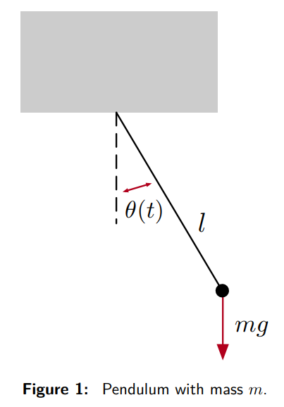
What is the system modeled in the pendulum motion example?

The pendulum motion system involves a mass m hanging from a weightless spring of length l. The angular position \theta(t) changes over time due to gravitational and frictional forces.

What is the equation describing the motion of the pendulum?

The motion of the pendulum is captured by the second-order ODE:

ml\ddot{\theta}(t) = -dl\dot{\theta}(t) - mg \sin\theta(t)

where \ddot{\theta}(t) is angular acceleration, \dot{\theta}(t) is angular velocity, m is the mass, g is the gravitational constant, l is the length, and d is the friction dissipation constant.

mass x angular acceleration = - frictional deceleration (prop. to velocity) - force of weight

What is the measurement equation for the pendulum example?

The measurement equation assumes that only the angular position is measurable: y(t) = \theta(t)

How is the system state represented in the pendulum example?

The system state is defined as:

x(t) = \begin{bmatrix} \theta(t) \\ \dot{\theta}(t) \end{bmatrix} \in \mathbb{R}^2

with the state equations:

\dot{x}(t) = \begin{bmatrix} \dot{x}_1(t) \\ \dot{x}_2(t) \end{bmatrix} = \begin{bmatrix} x_2(t) \\ -\frac{d}{m}x_2(t) - \frac{g}{l}\sin x_1(t) \end{bmatrix}

and the output equation: y(t) = \begin{bmatrix} 1 & 0 \end{bmatrix}x(t)

(previous equation of motion rearranged)

How were the state equations derived from the system state in the pendulum example?

The state vector is defined as:

x(t) = \begin{bmatrix} \theta(t) \\ \dot{\theta}(t) \end{bmatrix}

From the definition, the first state equation is:

\dot{x}_1(t) = \dot{\theta}(t) = x_2(t).

The second state equation is derived from the original motion equation:

ml\ddot{\theta}(t) = -dl\dot{\theta}(t) - mg \sin\theta(t),

substituting x_1(t) = \theta(t) and x_2(t) = \dot{\theta}(t) to get:

\dot{x}_2(t) = -\frac{d}{m}x_2(t) - \frac{g}{l}\sin x_1(t).

This results in the state-space representation:

\dot{x}(t) = \begin{bmatrix} \dot{x}_1(t) \\ \dot{x}_2(t) \end{bmatrix} = \begin{bmatrix} x_2(t) \\ -\frac{d}{m}x_2(t) - \frac{g}{l}\sin x_1(t) \end{bmatrix}.

What makes the pendulum system nonlinear and autonomous?

The system is nonlinear due to the presence of the \sin x_1(t) term in the state equation. It is autonomous because no external input forces are applied to the pendulum.

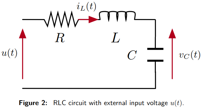
What is the system modeled in the electric circuit example?

The system involves a resistance R, an inductor L, and a capacitor C in series. An external voltage input u(t) is applied to the circuit.

What is the goal of the electric circuit modeling example?

The goal is to describe the behavior of the voltage across the capacitor v_C(t) and the current through the inductor i_L(t) using differential equations.

How is the voltage across the inductor expressed in the electric circuit example?

The voltage across the inductor is given by:

v_L(t) = L\frac{d i_L(t)}{dt}

How is the current through the capacitor related to the inductor in the circuit?

The current through the inductor equals the current through the capacitor:

i_L(t) = C\frac{d v_C(t)}{dt}

What is the differential equation governing the voltage across the capacitor in the circuit?

Combining Kirchhoff's voltage law and the inductor's and capacitor's behaviors, the second-order ODE is:

LC \frac{d^2 v_C(t)}{dt^2} + RC \frac{d v_C(t)}{dt} + v_C(t) = u(t)

What is the differential equation governing the voltage across the capacitor in the circuit? (derivation)

The second-order ODE for the voltage across the capacitor, v_C(t), is derived as follows:

1. The voltage across the inductor is expressed as:

v_L(t) = L \frac{d i_L(t)}{dt}

2. The current through the capacitor and inductor are equal, so:

i_L(t) = C \frac{d v_C(t)}{dt}

Substituting this into the expression for v_L(t) gives:

v_L(t) = LC \frac{d^2 v_C(t)}{dt^2}

3. The voltage across the resistor is given by:

v_R(t) = R i_L(t) = RC \frac{d v_C(t)}{dt}

4. Using Kirchhoff's Voltage Law, the total applied voltage u(t) equals the sum of voltages across the inductor, resistor, and capacitor:

v_L(t) + v_R(t) + v_C(t) = u(t)

Substituting the respective expressions for each voltage term:

LC \frac{d^2 v_C(t)}{dt^2} + RC \frac{d v_C(t)}{dt} + v_C(t) = u(t)

This is the second-order differential equation governing the voltage across the capacitor.

What is the state-space representation of the circuit's state?

The state vector is defined as: x(t) = \begin{bmatrix} v_C(t) \\ i_L(t) \end{bmatrix} \in \mathbb{R}^2

The state equations are: \dot{x}(t) = \begin{bmatrix} 0 & \frac{1}{C} \\ -\frac{1}{L} & -\frac{R}{L} \end{bmatrix} x(t) + \begin{bmatrix} 0 \\ \frac{1}{L} \end{bmatrix} u(t)

The output equation is: y(t) = \begin{bmatrix} 1 & 0 \\ 0 & 1 \end{bmatrix} x(t)

Why is the system described as linear but non-autonomous?

The system is linear because the state equations are linear functions of x(t) and u(t). It is non-autonomous because the external input u(t) is present.

What is the significance of the state-space representation in the circuit example?

The state-space representation transforms the second-order ODE into a first-order system of equations, explicitly separating the state evolution (state equation) and the measurable quantities (output equation).

What is the general form of a nonlinear, time-varying system in state space?

A nonlinear, time-varying system is represented in state space as:

\dot{x}(t) = f(x(t), u(t), t),

y(t) = h(x(t), u(t), t),

where x(t) is the state, u(t) is the input, y(t) is the output, and f and h are nonlinear functions of x(t), u(t), and possibly time t.

What does the dimension of the state in state space representation signify?

The dimension of the state n is referred to as the order of the system. It represents the number of state variables required to describe the system's dynamics.

What are the two forms of linear systems in state space representation?

1. Linear, time-varying systems:

\dot{x}(t) = A(t)x(t) + B(t)u(t),

y(t) = C(t)x(t) + D(t)u(t),

where A(t), B(t), C(t), D(t) are time-dependent matrices.

2. Linear, time-invariant systems (LTI):

\dot{x}(t) = Ax(t) + Bu(t),

y(t) = Cx(t) + Du(t),

where A, B, C, D are constant matrices.

What are the roles of x(t), u(t), and y(t) in state space representation?

- x(t) (state): Represents internal variables describing the system's evolution over time.

- u(t) (input): Denotes external actuation commands influencing the system.

- y(t) (output): Captures sensor measurements or observable quantities from the system.

When is a system considered time-invariant or autonomous in state space representation?

- Time-invariant: If the vector field f does not explicitly depend on time t.

- Autonomous: If the vector field f does not depend on t or u(t) (i.e., the system has no external inputs).

What are the key steps in deriving a system's state space representation?

1. Identify input variables u(t) (e.g., forces or voltages).

2. Determine output variables y(t) (e.g., measurable quantities).

3. Select state variables x(t) to describe the system's dynamics.

4. Derive the state equation: \dot{x}(t) = f(x(t), u(t), t) using physical laws.

5. Formulate the output equation: y(t) = h(x(t), u(t), t).

What is the physical significance of state variables?

State variables x(t) describe internal system dynamics. They are chosen to:

1. Capture energy storage (e.g., position, velocity, current, voltage).

2. Provide enough information, alongside inputs, to predict future behavior.

3. Represent the minimum number of variables needed to describe the system's state.

What laws are commonly used to derive state equations?

State equations are typically derived using:

- Newton's laws: For mechanical systems (forces and motion).

- Kirchhoff's laws: For electrical systems (currents and voltages).

What is the purpose of the output equation in state space representation?

The output equation y(t) = h(x(t), u(t), t) specifies measurable quantities, which may include:

- A subset of the state variables.

- A combination of state variables and inputs.

- Direct measurements of the system's outputs.

What is the purpose of linearization in control theory?

Linearization simplifies the analysis and design of controllers for nonlinear systems by approximating them with linear systems locally around a nominal trajectory or operating point. This allows leveraging well-established linear control methods.

A nonlinear, time-varying system is represented in state space as:

\dot{x}(t) = f(x(t), u(t), t),

y(t) = h(x(t), u(t), t),

From now on, the representation we will look at is the following vector field (n refers to number of states):

f(x(t), u(t)) = \begin{bmatrix} f_1(x(t), u(t)) \\ \vdots \\ f_n(x(t), u(t)) \end{bmatrix},

What is a nominal point or trajectory in the context of linearization?

A nominal point (x^*, u^*) or nominal trajectory (x^*(t), u^*(t)) represents a reference solution of the system’s equations that satisfies the dynamics \dot{x}^*(t) = f(x^*(t), u^*(t)). It serves as the baseline around which small perturbations are considered during linearization.

The nominal trajectory can be thought of as the ideal path that the system would follow in the absence of any disturbances or model mismatches. In reality, due to these factors, the actual trajectory of the system may deviate from the nominal trajectory.

A nominal point, denoted as (x*, u*), is a specific operating point for a system. It represents a steady-state condition where the system's state and input remain constant over time. This point is used as a reference point for the linearization of nonlinear systems

How is the state and input perturbed in linearization?

A perturbation is applied around the nominal trajectory (x^*(t), u^*(t)) such that:

x(t) = x^*(t) + x_p(t) and u(t) = u^*(t) + u_p(t),

where x_p(t) and u_p(t) represent small perturbations in the state and input, respectively.

We will now attempt to form a linear system modelling these pertubations.

What is the Taylor series expansion of the system’s vector field for linearization?

A nonlinear, time-varying system is represented in state space as:

\dot{x}(t) = f(x(t), u(t), t),

y(t) = h(x(t), u(t), t),

The vector field f(x, u) is expanded as:

f(x, u) = f(x^*, u^*) + \frac{\partial f}{\partial x}(x^*, u^*) x_p + \frac{\partial f}{\partial u}(x^*, u^*) u_p + \text{higher-order terms},

where the higher-order terms are neglected for small perturbations. This follows the Taylor series formula for multi-variate functions.

This is then used to derive a system for the pertubations. Full derivation is in the notes.

What is the resulting linearized system after applying the Taylor expansion for trajectories?

The linearized system around a nominal trajectory is given by (p standing for pertubations around the trajectory):

\dot{x}_p(t) = A(t)x_p(t) + B(t)u_p(t),

where:

- A(t) = \frac{\partial f}{\partial x}(x^*(t), u^*(t)) is the Jacobian of f with respect to x.

- B(t) = \frac{\partial f}{\partial u}(x^*(t), u^*(t)) is the Jacobian of f with respect to u.

f is a vector that consists of multiple functions.

How is linearization different for nominal operating points instead of trajectories?

For a nominal operating point (x^*, u^*) (instead of a trajectory), the linearization yields a time-invariant system:

\dot{x}_p(t) = Ax_p(t) + Bu_p(t),

where:

- A = \frac{\partial f}{\partial x}(x^*, u^*)

- B = \frac{\partial f}{\partial u}(x^*, u^*)

are constant matrices.

This is shown below:

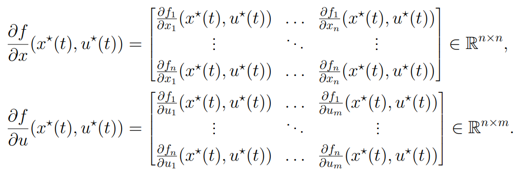
A = \frac{\partial f}{\partial x}(x^*, u^*) = \begin{bmatrix} \frac{\partial f_1}{\partial x_1} & \frac{\partial f_1}{\partial x_2} & \cdots & \frac{\partial f_1}{\partial x_n} \\ \frac{\partial f_2}{\partial x_1} & \frac{\partial f_2}{\partial x_2} & \cdots & \frac{\partial f_2}{\partial x_n} \\ \vdots & \vdots & \ddots & \vdots \\ \frac{\partial f_n}{\partial x_1} & \frac{\partial f_n}{\partial x_2} & \cdots & \frac{\partial f_n}{\partial x_n} \end{bmatrix}_{x = x^*, u = u^*},

B = \frac{\partial f}{\partial u}(x^*, u^*) = \begin{bmatrix} \frac{\partial f_1}{\partial u_1} & \frac{\partial f_1}{\partial u_2} & \cdots & \frac{\partial f_1}{\partial u_m} \\ \frac{\partial f_2}{\partial u_1} & \frac{\partial f_2}{\partial u_2} & \cdots & \frac{\partial f_2}{\partial u_m} \\ \vdots & \vdots & \ddots & \vdots \\ \frac{\partial f_n}{\partial u_1} & \frac{\partial f_n}{\partial u_2} & \cdots & \frac{\partial f_n}{\partial u_m} \end{bmatrix}_{x = x^*, u = u^*}.

Formulas for calculating A and B for systems using nominal trajectories instead?

Same as previous flashcard but instead uses x*(t) and u*(t)

What is the significance of linearization for control design?

Linearization allows designing controllers for the linearized system (e.g., feedback controllers) to regulate the system behavior near a nominal trajectory. However, this design is valid only locally due to the approximation of higher-order terms.

What is the linearization of the pendulum system around its nominal operating points?

The pendulum system is represented as:

f(x) = \begin{bmatrix} f_1(x) \\ f_2(x) \end{bmatrix} = \begin{bmatrix} x_2 \\ -\frac{d}{m}x_2 - \frac{g}{l} \sin x_1 \end{bmatrix},

where x_1 is the angular position and x_2 is the angular velocity. For linearization around a nominal point, the Jacobian matrix A is calculated as:

A = \begin{bmatrix} \frac{\partial f_1}{\partial x_1} & \frac{\partial f_1}{\partial x_2} \\ \frac{\partial f_2}{\partial x_1} & \frac{\partial f_2}{\partial x_2} \end{bmatrix} = \begin{bmatrix} 0 & 1 \\ -\frac{g}{l} \cos x_1^* & -\frac{d}{m} \end{bmatrix}.

The linearized system is given by (because B is zero due to no input):

\dot{x}_p(t) = A x_p(t).

For the two nominal operating points:

1. At x^* = \begin{bmatrix} 0 \\ 0 \end{bmatrix}:

A = \begin{bmatrix} 0 & 1 \\ -\frac{g}{l} & -\frac{d}{m} \end{bmatrix}.

2. At x^* = \begin{bmatrix} \pi \\ 0 \end{bmatrix}:

A = \begin{bmatrix} 0 & 1 \\ \frac{g}{l} & -\frac{d}{m} \end{bmatrix}.

The difference arises from the term \cos x_1^*, which reverses the gravitational force component. The small-angle approximation \sin x_1 \approx x_1 simplifies the system for x_1^* = 0, making the linearized behavior near the equilibrium predictable. This linearization highlights that the system dynamics depend significantly on the nominal point.