9. Population Growth

Population size def. 

the humber of individuals of the same species living in a defined geographical area

Population sizes change equation

(Births - deaths) + (immigrants - emigrants)

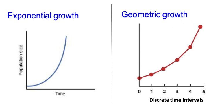
population growth models

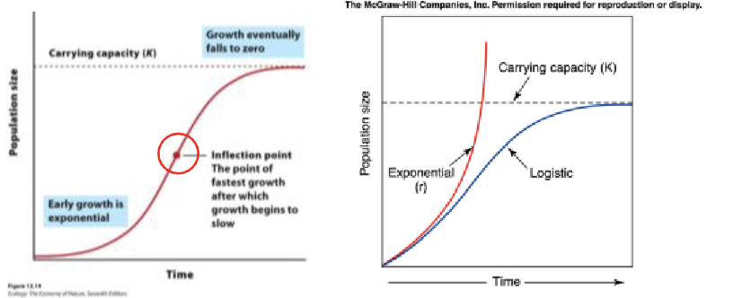
Geometric and exponential models describe population growth in an idealized environment with unlimited resources and good conditions

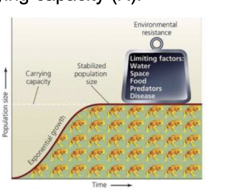
Carrying capacity

the max amount of individuals in a population due to limiting factors & resources

Population growth rate def.

the humber of new individuals that are produced per unit of time minus the number of individuals that die 

births - deaths

Intrinsic growth rate ( r ) def.

the highest possible per capita growth rate for a population (max. reproductive rates and min. death rates 

Closed population intrinsic growth rate ( r ) equation

r = b - d

r = birth rate - death rate

intrinsic growth rate ( r ) equation example

A population of 100 bats. In a year 80 are born and 60 die 

b = 80 / 100 = 0.8

d = 60 / 100 = 0.6

r = 0.8 - 0.6 = 0.2 

or 

80-60 / 100 = 0.2 

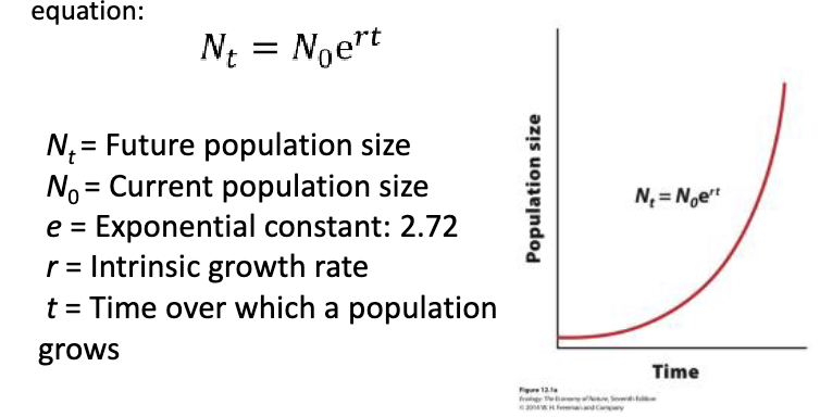
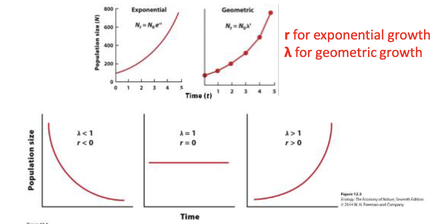
Exponential growth model def

A model of population growth in which the population increases continusouly at an expeoential rate; can be described by the equation Nt = Noe^rt 

Nt = Noe^rt  equation

Nt = future population size

No = Current population size

e = exponential constant 2.72

r - intrinsic growth rate

t - time over which a population grows 

G = rN equation

G = number of individuals added during any time interval

r = intrinsic growth rate b - d 

N = population size 

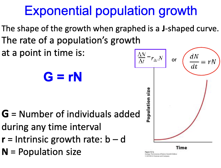
In exponential growth what is proportional

number of new individuals to size of population 

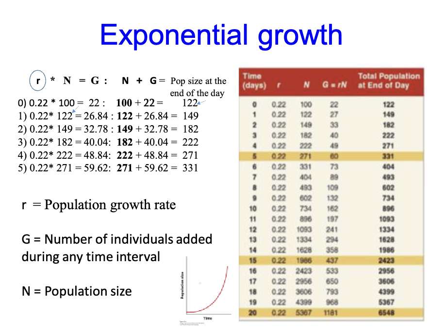
Exponential growth example

we have 100 ladybugs with r = 0.22 per day. How many individuals will be added per day? 

G = r x N

r = 0.22

N = 100

G = 0.22 × 100 = 22 individuals per day

New population size equation

N + G

G = number of individuals added during certain time interval

N = population size of the time interval

New population size equation example 

0) 0.22 100 = 22 : 100 + 22 = 122
1) 0.22 122 = 26.84 : 122 + 26.84 = 149
2) 0.22* 149 = 32.78 : 149 + 32.78 = 182
3) 0.22* 182 = 40.04: 182 + 40.04 = 222
4) 0.22* 222 = 48.84: 222 + 48.84 = 271
5) 0.22* 271 = 59.62: 271 + 59.62 = 331

Geometric growth model

Discrete time intervals / breeding seasons

expressed as ratio of a population’s size in one year to its size in the preceding year λ

λ: N1/No, N2/Na, etc

λ cannot be negative

λ > 1 population size has increased

λ = 180 / 100 - 1.8

λ < 1 population size has decreased

λ = 80 / 100 = 0.8 (lower than 1)

Geometric growth model time intervals

The size of a population after one time interval is:

N1 = N0λ
After two time intervals, the population size would be:

N2 = (N0λ)λ = N0λ² 
Or, more generally, after t time intervals

Nt = N0λ^t 

Geometric growth model time intervals example

Start with a population of 100 individuals.
Annual growth rate λ = 1.5
After 5 years the size of the population is:
N5= N0 x λ5 = 100 x 1.55 = 759
1.5×1.5×1.5×1.5×1.5 = 7.59

Comparing growth models 

Population decreasing λ < 1 and r < 0

Population constnat λ = 1 and r = 0

Population increase λ > 1 and r > 0

Density dependent controls def. 

effects increase as population grows; intraspecfic competition, predation, parasitism, and infectious disease.

Higher population size = food supply diminishes, compettion increases

Higher denstiy = infectious diseases spread more easily

Higher density = Preadators are attracted

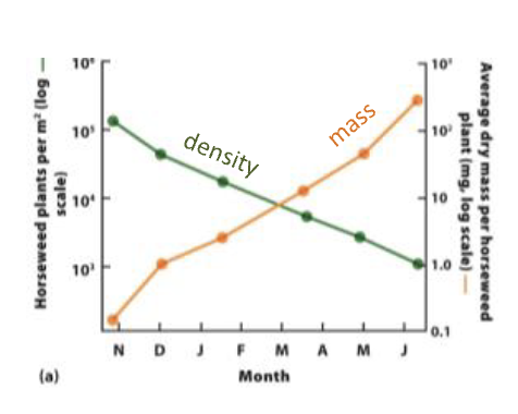
Desntiy depdednce in plants

Horseweed plants at a
density of 100,000 m2.
Over time, many individuals
died.
As density decreased, there
was a significant increase in
the weight of surviving
individuals

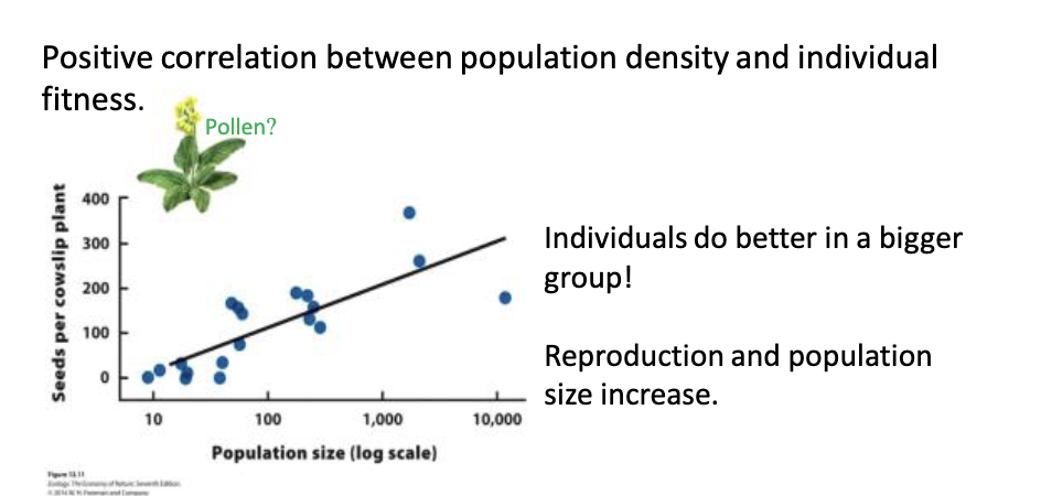
Postive density depdence def

rate of population growth can increase as popualtion desnity increases (allel effect)

postive ocrrelation between population density & indivdual fitness 

Density indepdent controls def.

Limit population size regardless of the population’s density

Cliamtic events (torandoes, floods, tempeatures, droguths, fire

birth and death rates do not change as density rises but sudeenly mortaitly rate increases and repodruvce rate decreases

Logistic growth model

The per captia rate of population growth approaches zero as the population size nears carrying capacity (K) 

Logistc growth model requation

dN/dt = rN (1 - N/K)

G = rN (K-N/K)

G = number of individuals added per unit of time

r = growth rate

N = number of individuals in the population at a given time (population size)

K = carrying capacity 

Carrying cacpacity (K) def

the maximum population size that can be supported by the envrioment

As population size increases

• resoruce shortages

• enviomrnetal limitations

• withing-sepcies compettion

• upper limit on population size

• not fixed, can change

S-shaped curve def

shape of curve when a poplation is graphed over time using the logtistc growth model

Inflection point def

the point on a sigmodial grwoth curve at which the population has its highest growth rate

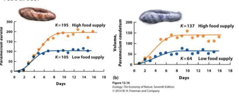
Two species of protists with a fixed amount of food each day.

Populations initially grew in size but eventually stabilized at
different carrying capacities depending on the available
resources.

A mammalogist estimates that there are N1 =
10,000 mice living in a large section of forest,
which she estimates has a carrying capacity (K) of
100,000. The population appears to have an
intrinsic growth rate (r) = 0.05 mice / mouse / year
What do you predict for G during this next year?
a) 45 mice
b) 50 mice
c) 450 mice
d) 500 mice
e) 4500 mice

G = rN (K-N/K)

r - 0.05

N = 10,000

K = 100,000

G = (0.05)(10,000) (100,000 - 10,000) / 100,000)

G = 450 mice

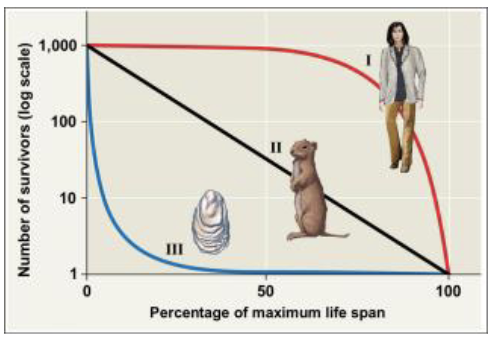
Survivorship Curves

Type I: Low mortality early in life

Type II: Sontant mortality

Type III: High mortality early in life

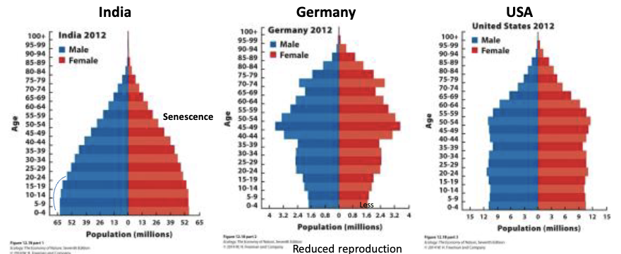
Age strucutre pyramids 

broad bases: growing population

Narrow bases: declining poulation

Straight sides: stable population

Life table 

Contain class - specfic survival and fecusintiy data

based on the number of female offspring per female

x = age class 

Nx = number of indivduals in each age

Sx = surival rate from one age

bx = the fecunigty of each age class (briths)

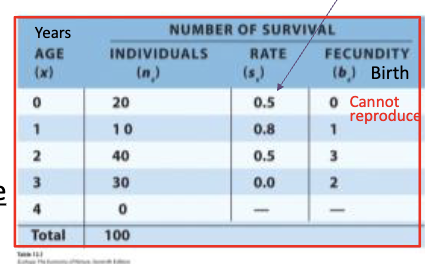
Life table calculations

Number surviving to next age class - nx x sx = 20 x - 0.5 = 10

Number of new off spring produced = nx x sx x bx = 10 × 0.5 × 1 = 10

λ: The number of individuals in a population after one time interval
divided by the initial number of individuals λ: N1/N0=112/100=1.12

Life table survivorship def

The probabilty of survving from birth to any later age class ( /x); surviorship in the first age class is always set at 1

example surviroship to the second year (I2) is calcuted as l2 = l1s1

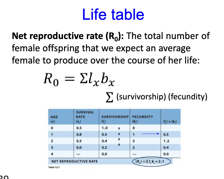
Life table newt reporeucte rat R0 def.

the total number of female offspring that we expect an averate female to produce over the course of her life

R0 = total lxbx

total = surivierhip fecundity