Biostatistics Exam 3
1/65
There's no tags or description
Looks like no tags are added yet.
Name | Mastery | Learn | Test | Matching | Spaced | Call with Kai |
|---|
No analytics yet
Send a link to your students to track their progress
66 Terms
Two sample design
Two groups
Each treatment group composed of independent, random sample units
Wild type vs. control, drug vs. placebo, where treatments are applied to separate and independent samples
Paired design
Two groups
Each sampled unit receives both treatments
Both treatments applied to every sampled unit
More powerful b/c control for variation among sampling units
Not as common
Two measurements from same sampling units —> converted to single measurement by taking difference between them
Examples (patient weight before and after hospitalization, effects of sunscreen on one arm vs placebo on another arm, effects of environment on identical twins raised under different socioeconomic conditions)
Estimating mean difference
From sample of di
d = after-before
Paired t-test
Used to test the null hypothesis that the mean difference of paired measurements equals a specific value
H0: mean change in antibody production after testosterone implants was 0 (mud=0)
HA: mean change in antibody production after testosterone implants was not 0
Paired t-test statistic
One paired samples reduced to single measurement (d)
Calculation is same as one-sample t-test
Can determine P with computer or statistical table
Fail to reject the null hypothesis that the mean change in antibody production after the testosterone implant is 0
Assumptions of paired t-test
Sampling units are randomly sampled from the population
Paired differences have a normal distribution in the population
Formal tests of normality
H0: sample has normal distribution
HA: sample does not have normal distribution
Should be used with caution
Small sample sizes lack power to reject a false null (Type II error)
Large sample sizes can reject null when the departure from normality is minimal and would not affect methods that assume normality
Shapiro-Wilk test
Evaluates the goodness of fit of a normal distribution to a set of data randomly sampled from a population
Most commonly used formal test of normality
Estimates mean and standard deviation using sample data
Tests goodness-of-fit between sample data and normal distribution (with mean, sd of the sample)
Pooled sample variance (s2p)
The average of the variances of the samples weighted by their degrees of freedom
Two-sample t-test
Simplest test to compare the means of a numerical variable two independent groups
Most commonly…
H0: mu1=mu2
HA: mu1 does not equal mu2
Assumptions of two-sample t-test
Each of two samples is a random sample from its population
Numerical variable is normally distributed in each population
Robust to minor deviations from normality
Need to run Shapiro-Wilk test on both samples
Standard deviation (and variance) of the numerical variable is the same in both populations
Robust to some deviation from this if sample sizes of two groups are approximately equal
Formal tests of equal variance
An F-test is sometimes used, but it is highly sensitive to departures from the assumption that the measurements are normally distributed in the population
Levene’s test performs better and is recommended
H0: variances of the two groups are equal
HA: variances of the two groups are not equal
Can be extended to more than two groups
What if variances in two groups are not equal?
Standard t-test works well if both sample sizes are greater than 30 and there is less than 3 fold difference in standard deviations
Welch’s t-test compares the means of two groups and can be used even when the variances of the two groups are not equal
Slightly less power compared to standard t-test
Should be used when the sample standard deviations are substantially different
Formulae are different than standard two-sample t-test
Correct sampling units
When comparing the means of two groups, an assumption is that the samples being analyzed are random samples
Often, repeated measurements are taken on each sampling unit
Makes the identification of independent units more challenging
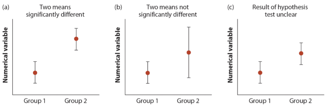
Fallacy of indirect comparison
Compare each group mean to hypothesized value rather than comparing group means to each other
Comparisons between two groups should always be made directly, not indirectly by comparing both to the same hypothesized value
Ex: since group 1 is significantly difference than zero, but group 2 is not, then groups 1 and 2 are significantly different from each other
Interpreting overlap in confidence intervals
Papers often report means and confidence intervals for two or more groups without running a two-sample t-test
t-distribution
Similar to standard normal distribution (Z), but with fatter tails
As the sample size increases the t distribution becomes more like the standard normal distribution
Has critical values like Z
Get values with computer or table
One-sample t-test
Compares the mean of a random sample from a normal population with the population mean proposed in a null hypothesis
H0: the true mean equals mu0
HA: the true mean does not equal mu0
Interpreting t-statistic
Compute P-value: probability of this t-statistic (or more extreme) given the null hypothesis is true
Using a stats table
Look up critical t-value
Observed value is within range of -/+ critical value
Data consistent with true null
Increasing sample size
Increasing sample size reduces standard error of mean
Uncertainty of estimate of mean
Larger sample sizes increase probability of rejecting a false null hypothesis (power)
If this null is really false, then the sample of 25 failed to detect a false null (Type II error)
Assumptions of one-sample t-test
Data are a random sample from the population
Variable is normally distributed in the population
Few variables in biology are exact match to normality
But in many cases the test is robust to departures from normality
Estimating other statistics
Emphasis on estimating the mean of a normal population
Spread of the sample distribution (standard deviation or variance)
Confidence limits for variance is based on the X2 distribution
Assumptions of calc confidence intervals for variance
Random sample from the population
Variable must have normal distribution
Formulas are not robust to departures from normality
Normal quantile plot
Compares each observation in the sample with its quantile expected from the standard normal distribution. Points fall roughly along a straight line if the data come from a normal distribution
Ignoring violations of normality
t-tests assume data are drawn from a population have a normal distribution
But can sometimes be used when data are not normal
Central limit theorem
When sample sizes are large the sampling distribution of means behaves roughly as assumed by t-distribution
Large sample size depends on shape of the distribution
If distributions of two groups being compared are skewed in different directions, then avoid t-tests even for large samples
If distributions are similarly skewed then there is more leeway
Ignoring violations of equal standard deviations
Two sample t-tests assume standard deviations in the two populations
If sample sizes are >30 in each group AND sample sizes in two groups are even, then even up to a 3x difference can be ok
Otherwise, use Welch’s t-test
Data transformations
A data transformation changes each measurement by the same mathematical formula
Can make standard deviations more similar and improve fit of the normal distribution to the data
All observations must be transformed
If two samples then they both must be transformed in same way
If used then usually best to back transform confidence intervals
Log transformation
Data are transformed by taking the natural log (ln) or sometimes log base-10 of each measurement
Common uses:
Measurements are ratios or products
Frequency distribution skewed to the right
Group having larger mean also has larger standard deviation
Data span several orders of magnitude
Other transformations
Arcsine (best use: proportions)
Square-root (counts)
Square (skewed left)
Antilog (skewed left)
Reciprocal (skewed right)
Nonparametric alternatives
A nonparametric method makes fewer assumptions than standard parametric methods do about the distributions of the variables
Can be used when deviations from normality should not be ignored, and sample remains non-normal even after transformation
Do not rely on parametric statistics like mean, standard deviation, variance
Usually based on ranks of the data points rather than the actual values
Sign test
Compares the median of a sample to a constant specified in the null hypothesis. It makes no assumptions about the distribution of the measurement of the population
Each measurement is characterized as above (+) or below (-) the null hypothesis
If the null is true, then you expect the half the measurements to be + and half to be -
Uses binomial distribution to test if the proportion of measurements above the null hypothesis is p = 0.5
Wilcoxian sign-ranked test
More power than standard sign test because information about the magnitude away from the null for each data point
But test assumes that population is symmetric around the median (i.e., no skew)
Nearly as restrictive as normality assumption, thus not recommended
Mann-Whitney U-Test
Nonparametric test for two samples
Compares the distributions of two groups. It does not require as many assumptions as the two-sample t-test
What if you have tied ranks?
Assign all instances of the same measurement the average of ranks that the tied points would have received
Mann-Whitney U-test further explained from office hours:
inability to do two sample t-test due to lack of normal distribution
e.g. right skew failed shapiro test for group 1 and group 2, but group 2’s distribution looks a bit different
takes all data points and ranks them from low to high
null is that distribution of ranks is equal in group 1 and group 2
sprinkling of black and green along the line would be equal visually
e.g. now imagine that right skew for group 1 and left skew for group 2
lowest is only black then some green, then you get to the highest and its mostly/all green with little black
this would show the alternative hypothesis that distribution of ranks is not equal
p<0.05
Assumptions of nonparametric tests
Still assume that both samples are random samples from their populations
Wilcoxian signed-rank test assumes distributions are symmetrical (big limitation-not recommended)
Rejecting null hypothesis of Mann-Whitney U-test means two groups have different distributions of ranks, but does not necessarily imply that means of medians of groups differ
To make this inference there is an assumption that the shapes of the distributions are similar
ANOVA
Analysis of variance (ANOVA) compares the means of multiple groups simultaneously in a single analysis
Tests for variation of means among groups
H0: mu1 = mu2 = mu3…mun
HA: mean of at least one group is different from at least one other group
Null assumption that all groups have the same true mean is equivalent to saying that each group sample is drawn from the same population
But each group sample is bound to have a different mean due to sampling error
ANOVA determines if there is more variance among sample means than we would expect by sampling error alone
Two measures of variation
Test statistic is a ratio:
True null: MSgroups/MSerror = 1
False null: MSgroups/MSerror > 1
Group mean square (MSgroups)
Proportional to the observed amount of variance among group sample means
Variation among groups
Error mean square (MSerror)
Estimates the variance among subjects that belong to each group
Variation with groups
ANOVA calculations
Sums of squares (SS) calculates two sources of variation (among and within groups)
Grand mean
Equal to a’ constant
Group mean square (MSgroups) is variation among
Group error square (MSerror) is variation among individuals in same group
F-ratio test statistic
Has pair of degrees of freedom
Numerator and denominator
Use to calculate P-value with stats table or computer
Variation explained
R2 measures the fraction of variation in Y that is explained by group differences
Assumptions with variation
Measurements in every group represent a random sample from the corresponding population
Variable is normally distributed in each of the k populations
Robust to deviations, particularly when sample size is large
Variance is the same in all k populations
Robust to departures if sample sizes are large and balanced, and no more than 10x differences among groups
Alternatives with variation
Test normality with Shapiro-Wilk and test equal variances with Levene’s test
Data transformations can make data more normal and variances more equal
Nonparametric alternative: Kruskal-Wallis test
Similar principle as Mann-Whitney U-test
Planned comparisons
A planned comparison is a comparison between means planned during the design of the study, identified before the data are examined
In circadian clock follow-up study, the planned (a priori) comparison was difference in means between knee and control group
Unplanned comparisons
Comparisons are unplanned if you test for differences among all means
Problem of multiple tests (increasing probability of Type I error) should be accounted for
With the Tukey-Kramer method the probability of making at least one Type I error throughout the course of testing all pairs of means is no greater than the significance level
Tukey-Kramer method
Works like a series of two-sample t-tests, but with a higher critical value to limit the Type I error rate
Because multiple tests are done, the adjustment makes it harder to reject the null
Kruskal-Wallis post-hoc test
Suppose that your data…
Fail normality even after transformation
Generate a significant Kruskal-Wallis result
So the interpretation is that the distribution of ranks differs for at least one group. But which one?
Should not use Tukey-Kramer, which is a parametric test
Dunn’s test
The appropriate analysis for a post-hoc analysis of groups following a significant Kruskal-Wallis result
Will compare all possible pairs of groups while controlling for multiple tests
Correlation
When two numerical variables are associated then they are. correlated
Correlation coefficient
The correlation coefficient measures the strength and direction of the association between two numerical variables
AKA linear correlation coefficient or Pearson’s correlation coefficient
Correlation coefficient (statistic), r
Population correlation coefficient (parameter), p
Ranges from -1 to 1
Possible that two variables can be strongly associated but have no correlation (r=0)
Non-linear association
Standard error of correlation coefficient
Sampling distribution of r is not normally distributed, so SEr isn’t used in calculating the 95% CI
Approx. confidence. interval of correlation coefficient
Involves conversion of r that includes natural log, and then back conversion
Correlation assumptions
Random sample from the population
Bivariate normal distribution
Bell shaped in two dimensions rather than one
Deviations from bivariate normality
Transform data (both variables same way)
Nonparametric test (Spearman’s rank correlation); skipping
ANOVA as a linear model
Linear model Y=+A
Y: response
: grand mean (constant)
A: treatment
Circadian clock study: SHIFT = CONSTANT + TREATMENT
H0: treatment means are all the same
SHIFT = CONSTANT
HA: treatment means are not all the same
SHIFT = CONSTANT + TREATMENT
Even if the null hypothesis is true, however, the treatment means will be different due to sampling error
Thus, the full model (with TREATMENT) will be a better “fit” to the data
The F-ratio is used to test whether including the treatment variable in the model results in a significant improvement in the fit of the model to the data
Compared with the fit of the null model lacking the treatment variable
ANOVA linear model: RESPONSE = CONSTANT + EXPLANATORY
Extending for multiple explanatory variables
RESPONSE = CONSTANT + EXP1 +EXP2 + EXP1 * EXP2
Design is called a two-way ANOVA or two-factor ANOVA
Two-factor outcomes
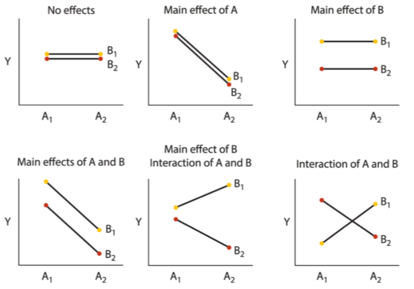
Assumptions of two-factor ANOVA linear models
The measurements at every combination of values for the explanatory variables are a random sample from the population of possible measurements
The measurements for every combination of values for the explanatory variables have a normal distribution in the corresponding population
The variance of the response variable is the same for all combinations of the explanatory variables
Correlation vs regression
Correlation measures the aspects of the linear relationship between two numerical variables
Regression is a method that predicts values of one numerical variable from values of another numerical variable
Fits a line through the data
Used for prediction
Measures how steeply one variable changes with the other
Linear regression
The most common type of regression
Although there are non-linear models (e.g., quadratic, logistic)
Draws a straight line through the data to predict the response variable (Y, vertical axis) from the explanatory variable (X, horizontal axis)
Fitting the “best” line
You want a line that gives the most accurate predictions of Y from X
Least-squares regression: line for which the sum of all the squared deviations in Y is the smallest
Formula for the line
Y = a + bX
a is the Y-intercept; b is the slope
The slope of a linear regression is the rate of change in Y per unit X
Also measures direction of prediction
Positive: as X increases Y increases
Negative: as X increases Y decreases
Calculating intercept
Once slope is calculated, getting intercept is straightforward because the least-squares regression always goes through point (X, Y)
Plug mean values into line formula: Y = a + bX
Rearrange to solve for intercept: a = Y - bX
Samples vs populations
The slope (b) and intercept (a) are estimated from a sample of measurements, hence these are estimates/statistics
The true population slope () and intercept () are parameters
Regression assumes that there is a population for every value of X, and the mean Y for each of these populations lies on the regression line
Predicting values
Now that you have the regression line you can predict values of Y for any specified value of X
Predictions are mean Y for all individuals with value X
Designated Y, or “Y-hat”
How well do data fit line?
The residual of a point is the difference between its measured Y value and the value of Y predicted by the regression line
Residuals measure the scatter of points above and below the least-squares regression line
Can be positive or negative
Variance in residuals (MSresidual) quantifies the spread of the scatter
Residual mean square
Analogous to error mean square in ANOVA
Used to quantify the uncertainty of the slope
Two types of predictions
Predict mean Y for a given X
E.g., what is the mean age of all male lions whose noses are 60% black?
Predict single Y for a given X
E.g., how old is that lion over there with a 60% black nose?
Both predictions give the same value of Y, but they differ in precision
Can predict mean with more certainty than a single value
Confidence bands measure the precision of the predicted mean Y for each value of X.
Prediction intervals measure the precision of the predicted single Y-values for each X
ANOVA (F) approach
Recall two source of variation in ANOVA
Among groups (MSgroups)
Within groups (MSerror)
In regression framework:
Deviations between the predicted values Yi and Y
Analogous to MSgroups
Deviations between each Yi and its predictive value Yi
Analogous to MSerror
Using ANOVA approach will generate the same P-value as the t-test approach
Can be used to measure R^2: the fraction of the variation in Y that is “explained” by X
R^2 = SSregression/SStotal
Regression toward the mean
Regression toward the mean result when two variables measured on a sample of individuals have a correlation less than one. Individuals that are far from the mean for one of the measurements will, on average, lie closer to the mean for the other measurement
Cholesterol measurements before and after drug
Solid line: linear regression
Dashed line: one-to-one line with slope of 1
Assumptions of linear regression
At each value of X:
There is a population of Y-values whose mean lies on the regression line
The distribution of possible Y-values is normal (with same variance)
The variance of Y-values is the same at all values of X
The Y-measurements represent a random sample from the possible Y-values
Detecting issues
Outliers
If only one (or a low number) then it may be reasonable to report regression with and without outlier
Nonlinearity can be detected by inspecting graphs
Non-normality and unequal variances can be inspected with a residual plot
Residual plot: residual of every data point (Yi - Yi) is plotted against Xi
If assumptions of normality and equal variances are met then there should be a roughly symmetric cloud above/below horizontal line at 0