AP Stat Last Minute Cram

What to describe when asked “Describe the Distribution” or “Compare the distribution”

SOCV+ Context—(Shape, Outliers, Center, Variability)

Compare Center and Variability when asked to compare different distributions or data sets.

Describe Shape in Context

The distribution of (context) is (shape) with a peak at (highest point) and gaps between (gap)

Ex. The distribution of the exam scores is roughly symmetrical with a peak at 75 and gaps between 50 and 60.

Describe Outliers in Context

There seems to be outliers at (values)

Ex. There seem to be outliers at 95 and 20 in the exam scores distribution.

Describe Center in Context

The (mean/median) of the distribution is (mean/median + units).
if symmetric—use mean
if skewed—use median

Ex.The mean of the distribution is 75 points. (If skewed, use median instead.)

If asked to compare: Compare which is greater to that which is lesser

Describe Variability in Context

The distribution of (context) has a (SD/IQR/Range + units).

Ex.The distribution of the exam scores has a standard deviation of 10 points.

If asked to compare: Compare which distribution varies more

Interpret SD

“The (context) typically varies by about (SD + unit) from the mean of (mean+unit)”

Parameter

A number(or statement) that describes a population

Statistic

A number(or statement) that describes a sample

5 Number Summary

Minimum

Q1(25th Percentile)

Median

Q3(75th Percentile)

Maximum

2 Ways to Describe Location

Percentiles or Standardized Scores(z-scores)

Interpret a Z-Score

“(context) is (z-score) standard deviations (above(+)/below(-)) the mean of (μ+units)

Addition/Subtraction of Data

Shape- No change

Center/Location-±a

Variability- No Change

Multiplication/Division of Data

Shape- No change

Center/Location-x/÷ b

Variability-x/÷ b

Density Curves

models the distribution variable with a curve that:

• is always above the horizontal axis

• has exactly an area of 1 under it

Mean of a Density curve- Point at which the curve would balance if made of a solid material

Median of a Density curve- is the point that divides the area under the curve in half

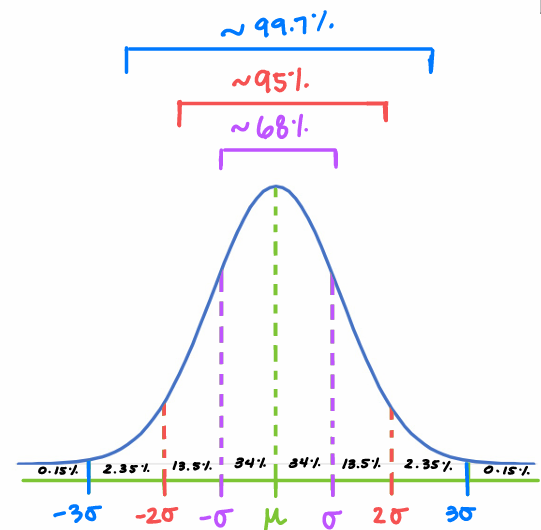
Approximately Normal/Normal Curve

Roughly symmetric, single-peaked, bell-shaped density curve

Normal Dist. specified by 2 parameters: mean & SD

Empirical Rule

68-95-99.7 Rule

How to describe a scatterplot

Direction:(Positive/Negative/None)

Unusual Feature:(Outlier)

Form:(Linear/Nonlinear)

S:(Weak/Moderate/Strong)

*Describe Direction+Strength using correlation( r ), if given

Interpret a Scatterplot

“There is a (strength), (correlation), (form) relationship between (explanatory variable) and (response variable). There does/doesn’t seem to be unusual features in this relationship.(If yes, describe)”

Ex. There is a strong, positive, linear relationship between studying time and test scores. There doesn’t seem to be unusual features in this relationship.

Interpret Correlation( r )

“The correlation of r= ( r ) confirms that the linear association between (explanatory variable) and (response variable) is (positive/negative) and (weak/moderate/strong).”

Interpret Residuals—(Actual-Predicted)(y-ŷ)

“The actual (y-context) was (residual value) (above/below) the predicted value for x=(# in context)”

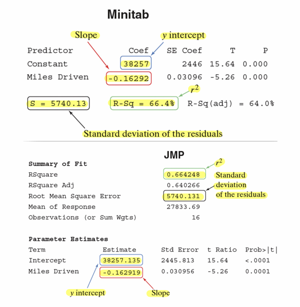
Interpret Slope(b)

“For every increase in (x-context) the predicted (y-context) (increases/decreases) by (slope unit of y).”

Interpret y-int(a)

“When (x-context) is 0, the predicted (y-context) is (y-int).”

Interpret Standard Deviation(In terms of LSRL)

“The actual (y-context) is typically about (s+unit) away from the number predicted by the LSRL with x=(context)

Context of Coefficient of Determination(r²)

“About (r²)% of the variability in (y-context) is accounted for by the LSRL at (x-context)

LSRL(Least Squares Regression Line) Equation

ŷ=a+bx

ŷ=predicted y

a=y-int

b=slope

x=explanatory variable

To find LSRL Eq. on Calc- Stat>Calc>8:Lin Reg(a+bx)

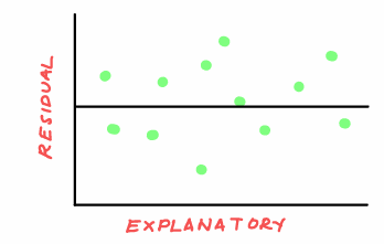
Residual Plot

Identifies if a Linear Model is appropriate

Appropriate if no leftover curved pattern

To find a & b

b=r * S_y/S_x a=ȳ-bx̄

Extrapolation

Explanatory Variables that are outside of the range of data which the LSRL was calculated

Influential Points

Can greatly affect correlation and regression calculaltions

Outliers

Out of pattern(large residuals)

High Leverage

Very large x-values

To tell if the Power Model is the best fit

Option 1: Raise the values of the explanatory variable by an integer, p

Option 2: Take the pth root of the response variable

To tell if the Exponential or Logarithmic Models are the best fit

Take the logarithm(log or ln) of one or both variables

Computer Generated Values

How to choose an SRS

Label, Randomize, Select

Must Be Without Replacement

Stratified Random Samplling

Taking a random sample from each strata(group)

More Precise Estimate

Cluster Sampling

Randomly select entire clusters- all individuals in the selected clusters are part of the sample

Saves time and money

Systematic Random Sample

Choose a k value, randomly select a starting value from 1 to k, choose every kth individual from the starting individual

Convenience Sampling

Choose individuals that are easiest to reach-BIAS

Voluntary Sampling

Individuals choose to be a part of the study b/c of open invitation-BIAS

Undercoverage

When some members of the population are less likely to be chosen or cannot be chosen in a sample

Nonresponse

When an individual chose for the sample can’t be contacted

Response Bias

When there is a systematic pattern of inaccurate answers to a survey question

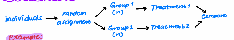
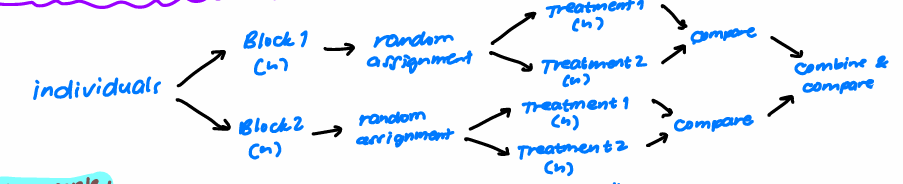
Completely Randomized Design-Experiments

Randomized Block Design

Observational Study

Observes individuals and measures variables of interest but observes without influencing the response

Experimental Study

Deliberately imposes treatments on individuals to measure their responses

Matched Pairs Design

Uses blocks of size 2; twins especially

Statistically Significant

The observed results of a study are too unusual to be explained by chance alone

Probability for Statistical Significance

%<= 5% means something is statistically significant

Process of Identifying the Percentage(p-value)

1. Identify the difference in mean

2. Make a simulation and dotplot

3. Identify how many dots are greater of equal to the difference in mean from step 1

4. Calculate the percentage of how many dots are greater than or equal to the mean difference

5. Compare to the 5% rule and state if the study is statistically significant or not in the context of the problem

Scope of Inference

Random Selection of individuals allow inference about the population from which the individuals were chosen

Random Assignment of individuals to groups allows inference about cause and effect

P(A)

number of outcomes in event A/total number of outcomes in sample space

Complement Rule

P(A^c)=1-P(A)

Addition Rule for Mutually Exclusive Events

P(A U B)= P(A) + P(B)

General Addition Rule

P(A U B)= P(A) + P(B) - P(A ∩ B)

Conditional Probabilities(“given that”)

P(A|B) = P(A ∩ B) / P(B) = P(both events occur)/P(given event occurs)

Independent Events

P(A) = P(A|B^c)=P(A|B)

General Multiplication Rule

P(A ∩ B) = P(A) * P(B|A)

Multiplication Rule for Independent Events

P(A ∩ B) = P(A) * P(B)

“At least one” Probability Rule

P(at least one)=1-P(none)

Law of Large Numbers

If we observe more and more trials of any random process, the proportion approaches the true probability

Mutually Exclusive

No event can happen at the same time

Simulation

Imitates a random process in such a way that simulated outcomes are consistent with real-world outcomes

Simulation process:

1) Describe how you will simulate one trial(one repetition)

2) Perform many trials(repetitions)

3) Use the result to answer the question

Conditional Probability

Probability that one event happens given that another event is known to have happened

Independent Events

If knowing whether or not one event has occurred does not change the probability that the other event will happen

Mean/Expected Value

μX​=E(X)=Σxi​P(xi​)

Discrete Random Variable

Uses summation to calculate probabilities and means

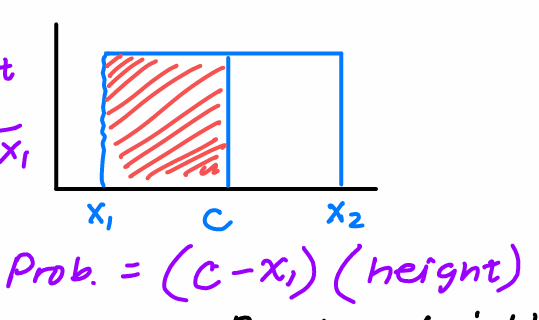
Continuous Random Variable

Probabilities are areas under a density curve

Height of Density Curve

1/X₂-X₁

Probability of C

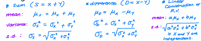
Combining Random Variables

Independent Random Variables

When x cannot hep or predict the value of y

Knowing the value of one variable does not change the probability of the other variable

Variance

σ²

Binomial Random Variables

When you have a fixed number of independent trials with the same probability of success

Conditions for Binomial Setting

BINS

Binary-”success” or “fail”

Independent-Knowing the outcome of one trial does not or tell us anything about the outcome of other trials. Or 10% Cond.

Number- fixed n number of trials

Same Probability- same probability p for every trial

10% Condition

If a binomial setting is not independent, we can use the 10% condition to treat each individual as independent

sample<=.1(population)

n<=10%N

Large Counts Condition

Helps us identify that the probability distribution of X is approximately Normal

n(p)>=10

n(1-p)>=10

Binomial Probability

P(X=x)=(nCx) (p)^x(1-p)^n-x

Mean(Expected Value)-Binomial

E(x)=np

SD-Binomial

\sqrt{np\left(1-p\right)} =σ_x

Geometric Random Variable

When you're counting the number of trials until the first success

Probability-Geometric

P(X=x)=(1−p)x−1p

Mean-Geometric

μ=p/1​

SD-Geometric

\frac{\sqrt{1-p}}{p} = σ

Shape of Geometric Distribution

Always right-skewed when small sample size

-shape is right-skewed, p<.5

-shape is left-skewed, p>.5

-shape is approximately normal, p=.5

Interpretation of Probability

“There is a (probability/percentage) chance/probability of (context)”

Interpretation of Mean

“If many, many (unit) were randomly selected, the average (context) is about (μ + unit)”

Interpretation of SD

“If many, many, (unit) were randomly selected, the (context) typically varies by about (σ + unit) from the mean of (μ + unit)”

Describing Random Variable(Discrete, Continuous, Binomial, or Geometric)

Describe the Shape, Center, & Variability

Population Distribution

Values of ALL individuals in a sample

Sampling Distribution

Values of ALL POSSIBLE samples of the same size from the same population

Unbiased Estimator

If the center(μp̂ or μx̄) in equal to the true value of the parameter(p or μ)

Central Limit Theorem

If the population distribution is not Normal, but the sample size is large enough(n>=30), the sampling distribution is approx. Normal by CLT

Point Estimate

A chosen statistic(p-hat, x-bar, S_x) that will provide a reasonable estimate about the parameter

A+B/2

Margin of Error Strength

Confidence Level +; ME +(wider intervals)

Sample Size +; ME -(narrower intervals)

How to make a Confidence Interval(One Sample)

Choose: One-Sample z interval for p

Conditions: Random, 10%, Large Counts

Calculate: Stat>Tests>1-PropZInt
x:n(p-hat)
n:sample size
c-level:c%

Conclude: Interpret

How to make a Confidence Interval(Two Sample)

Choose: Two-Sample z interval for p₁-p₂

Conditions: Random, 10%, Large Counts (For Both Samples)

Calculate: Stat>Tests>2-PropZInt
x:n(p-hat)
n:sample size
c-level:c%

Conclude: Interpret

Convincing Evidence in Confidence Intervals

(+,+)-1st proportion is greater

(-,-)-2nd proportion is greater

(+,-)- No convincing evidence of a difference b/c interval contains 0

Interpretation of a Confidence Interval

We are (c%) confident that the interval from A to B captures the p=true proportion of [parameter in context].