STAT 230 MIDTERM 2

EAT DOWN OK AMELIA AND DONT CRY OR KILL YOURSELF LIFE IS ROBLOX

Observed

Xijk

What is xijk?

observed value for the kth observation under the ith level of factor A and jth level of factor B

ai

effect of the ith level of factor A

μ

grand mean

Bj

effect of the jth level of factor B

(aB)ij

the interaction effect between level i of factor A and level j of Factor B

eijk

error/residual

C

Unknown true values are constant

A

components go together to make xijk by adding them

Z

The errors have a mean of zero. eg. E{εijk} = 0

S

errors (εijk) come from the same distribution, with

common standard deviation

I

errors are independent (eg. there is no relationship

between ε111 and ε112)

N

the distribution of εijk is Normal

Two assumptions about unknown true values

C and A

Four assumptions about errors:

Z, S, I, and N

SSCorrected Total =

 SSTotal − SSMean

√MSE =

whatever is the SD for this analysis. This is the estimate

of σε, the standard deviation of the ε’s

Hypotheses to test in a BF[1] design

H0 : α1 = α2 = · · · = αg = 0

vs.

Ha: At least one αi is different from the others

Test H0 for BF[1]

F-ratio

F-ratio = MSgroup/MSError = Variability due to group/Variability due to error = (One estimate of

chance error variability + Estimate of variability due to groups)/Another estimate

of chance error

MSError

quantifies variability due to error

η2

 interpreted as the percent of the

variability in the response that can be explained..

η2model =

SSexplained/ SSCorrectedTotal

η2FactorA=

 SSFactorA/SSCorrectedTotal

η2p

calculated to quantify the percent of the

variability explained by a single effect AFTER controlling for the variability explained by other factors:

η2p,FactorA =

SSFactorA/(SSFactorA + SSE)

where SSE is the SS for the error used to test Factor A

For BF[1] models, η2 =

η2p

Why randomize:

Protect against bias and confounding

2 Allows us to use probability and sampling distributions when

analyzing the data.

Balance refers to

the presence of equal treatment group size

Partition

 a way of sorting them into groups.

Factor

a meaningful partition of the observations

To find power, we need:

1 α (significance level)

2 n (observations per group)

3 I (number of groups)

4 values for α1, α2, . . . , αI

5 estimate of σ2

F-test does NOT

help you see which means are different or best.

comparison is

a measure of distance between means for two

groups of observed values.

What do we use if we want to check if the true difference equal to zero?

hypothesis test

What do we use if we want to check if the range of plausible values for true difference

CI

 two groups for comparison

µ1. − µ2.

3 groups for comparison

µ1. − µ2.

µ1. − µ3.

µ2. − µ3.

5 groups for comparison

µ1. − µ2.

µ1. − µ3.

µ2. − µ3.

µ1. − µ4.

µ2. − µ4.

µ3. − µ4.

µ1. − µ5.

µ2. − µ5.

µ3. − µ5.

µ4. − µ5.

Family-wise (Type I) error rate

The chance of at least one ___error among a ____

of tests, assuming there are no differences in the group means.

“contrasts” of the form c1µ1. + c2µ2. + ... + cIµI.

µ1. − (µ2. + µ3. + µ4. + µ5/4) ⇒ 1 -.25 -.25 -.25 -.25

orthogonal)

perpendicular/non-overlapping information. Totally distinct comparisons

can use a set of orthogonal contrasts to

split the SS for a factor into pieces, one piece for each contrast

Looking at multiple factors simultaneously allows us to:

1 Study the factors in one experiment instead of multiple experiments

2 Study how conditions interact

Two factors are crossed if

all possible combinations of the factors’ levels occur in the design.

Interaction

the effect of factor A on the response changes for different values of factor B.

BF[2]

yijk = µ + αi + βj + (αβ)ij + εijk

Three Null Hypotheses

H0: The mean wear for the 2 filler types is the same ← check main

effect for filler

–OR–

H0: α1 = α2 = 0

H0: The mean wear for the 3 proportions is the same ← check main

effect for filler

–OR–

H0: β1 = β2 = β3 = 0

H0: Proportion and Filler do NOT interact ← check interaction effect

H0: (αβ)11 = (αβ)12 = (αβ)13 = (αβ)21 = (αβ)22 = (αβ)23 = 0

Assessing the interaction requires

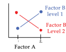
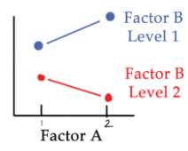
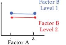
a response and two crossed factors Use an interaction plot

BF[2] Decomposition: Observed values

= Cell means + Residuals

BF[2] Decomposition: Cell means

estimated mean effect = factor level mean - grand mean

BF[2] Decomposition: Interaction effect

= cell mean - (grand mean + factor A effect + factor B effect)

The meaning of a main effect changes

if there is a significant interaction.

If interaction IS significant

Compare treatment means (are main effects meaningful)

If interaction is NOT significant

Evaluate and interpret main effects

p value for interaction is 0.01

p value for factor B is 0.90

pvalue for interaction is 0.01

p value for factor B is 0.01

p value for interaction is 0.90

pvalue for factor B is 0.20

Replication is important because

1 gives more precision to our estimates of model parameters

2 gives us information about the errors εij, which then allows us to make inference about model parameters.

what if there there is not replication?

Hope that the prop×filler interaction is non-existant/non-significant

if there is no interaction effect

MSinterax is just an estimate of σ2 (i.e., MSinterax ∼= σ2) . . . just run the model with no interaction term

UNBALANCED DATA:

Standard formula for estimating model parameters are often invalid

Order of the factors in the model affects SS, MS, and F-tests

Type I SS

gives first term in the model the chance to “explain” as much of the variability as possible, with 2nd, 3rd, and later terms a chance to explain what is leftover (Type I SS aka “Sequential SS")

Type III SS

which treats each term as if it were last in the model. That is, what is unique about this term after explaining all others (aka “SS Last”)

Type II SS

which gives the effect of each main effect in the presence of all other main effects, but before the two-way interaction(s); then it gives the effect of the interactions in the presence of the main effects and any other interactions of the same order.

For Type III and Type II SSModel /=

SSGender + SSType + SSInteraction