SNP, GWAS, and post-GWAS

Genome wide association studies (GWAS)

• Identify associations between genetic variations (loci) and traits (including diseases).

  • Test for differences in the frequency of genetic variants between individuals who are ancestrally similar but differ phenotypically.

• Genetic variations:

  • Single nucleotide polymorphism (SNP) → most common.

  • Copy number variants.

  • Large sequence variations.

Sinlge nucleotide polymorphism (SNP)

• Most common genetic variation (~90% of human variation).

• Single base pair change (substitution, insertion, or deletion).

• Location:

  • Coding: may change protein sequence.

  • Non-coding (majority): may affect gene expression, timing, or location.

SNP database

NCBI Short Genetic Variation database (dbSNP) catalogs short variations in nucleotide sequences for humans.

Major and minor allele

• Major allele is the most common variant found in a population, while the minor allele is the less common or rarer variant at that same position.

  • Minor allele frequency (MAF).

  • MAF > 1% → common SNP.

  • MAF < 1% → rare SNP.

• Major and minor alleles are population-specific.

• Focus often on the minor allele because minor alleles are crucial for identifying disease risks and studying genetic selection.

Synonymous vs. nonsynonymous SNPs

• Synonymous SNPs:

  • Do not change the amino acid sequence of a protein.

  • Silent change.

• Nonsynonymous SNPs:

  • Potentially alter protein structure and function.

• This distinction arises because the genetic code is redundant, with multiple codons sometimes coding for the same amino acid.

Missense vs. nonsense SNPs

• Missense and nonsense SNPs are both nonsynonymous mutations.

  • Change the amino acid sequence.

• Missense mutation:

  • Results in a different amino acid being incorporated into the protein.

  • It will alter the protein’s structure and function.

• Nonsense mutation:

  • This changes from a sense codon to a premature stop codon.

  • This leads to a truncated and often non-functional protein.

Linkage disequilibirum (LD) blocks

• LD = non-random association of genes.

  • There is a pattern.

• Sets of nearby SNPs on the same chromosome are inherited together in blocks.

• Haplotype/LD block:

  • A group of alleles that are co-inherited as a single block.

  • LDTools: LDHap, LDMatrix, etc.

Tag SNPs

• A few SNPs are enough to identify the haplotypes in a block uniquely.

  • Haplotype: a group of alleles/variants on the same chromosome that are inherited together.

• Reduce the number of SNPs required to examine the entire genome for association with a phenotype.

Methods other than measure SNPs

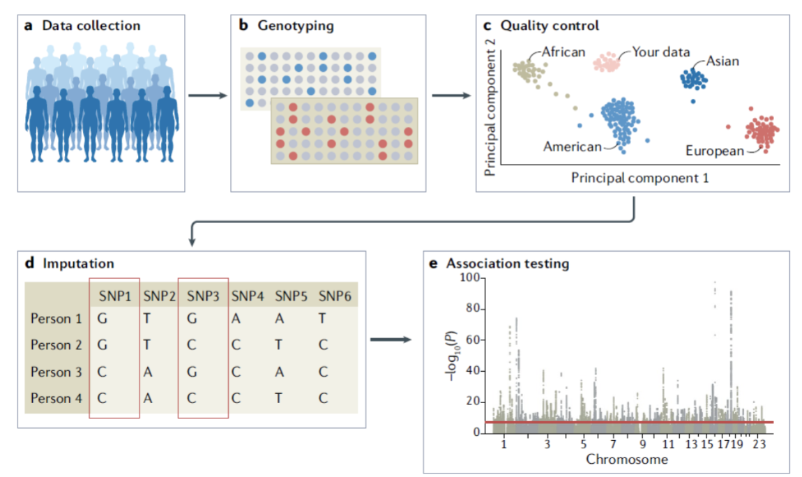
• Genotyping: targets known SNPs at specific sites (e.g., SNP arrays), cheaper, limited to pre-selected variants.

• DNA sequencing: reads entire DNA, finds known & novel SNPs (via variant calling → VCF), more data, more expensive.

How to do SNP selection (genotyping)

• Identify DNA regions of interest.

• Identify patterns of SNPs that are inherited together on a chromosome.

  • HapMap project: tested the association of millions of SNPs across multiple populations → produced the SNP panels that are used today.

• Select tag SNPs that can represent a block of associated SNPs.

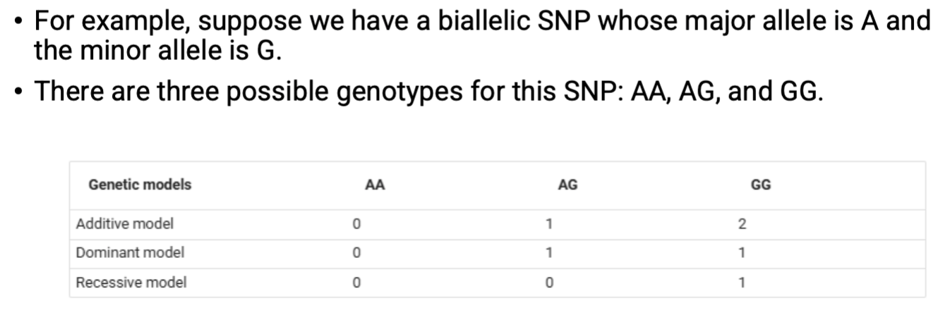
SNP genotype models

• SNP genotypes can be coded differently based on genetic models.

  • Additive model (ADD) → commonly used.

  • Dominant model (DOM).

  • Recessive model (REC).

• SNP genotypes are commonly coded as 0, 1, or 2 to represent the number of copies of the minor allele.

  • 0 → homozygous dominant (e.g., AA).

  • 1 → heterozygous (e.g., Aa).

  • 2 → homozygous recessive (e.g., aa).

Genotype/haplotype phasing

• Current technology gives genotypes but not haplotypes.

• The process of determining which alleles are located on the same chromosome, i.e., the haplotype.

• Phasing tools: SHAPEIT5, BEAGLE5.5.

GWAS association tests

• Chi-square / case-control: simple test, no confounders.

  • No confounders = assumes no other factors (e.g., age, ancestry) affect the association between a variant and a trait.

• Linear regression: continuous traits (height, BMI, blood pressure).

• Logistic regression: binary traits (disease yes/no).

• Linear mixed models: account for relatedness among individuals.

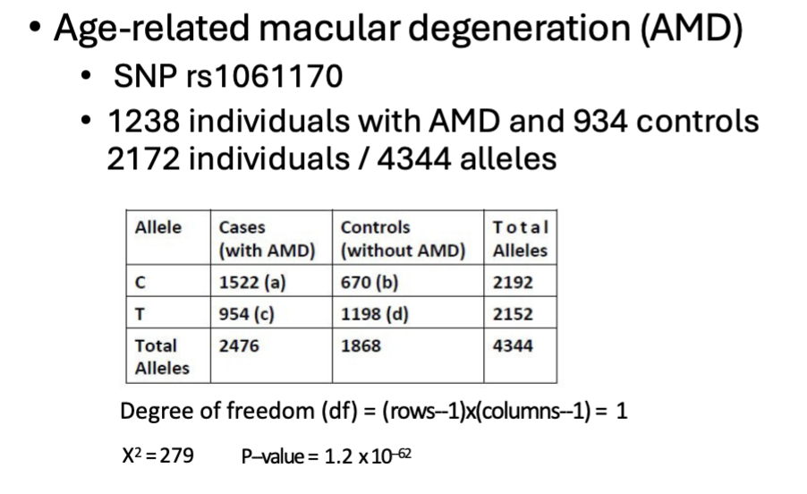
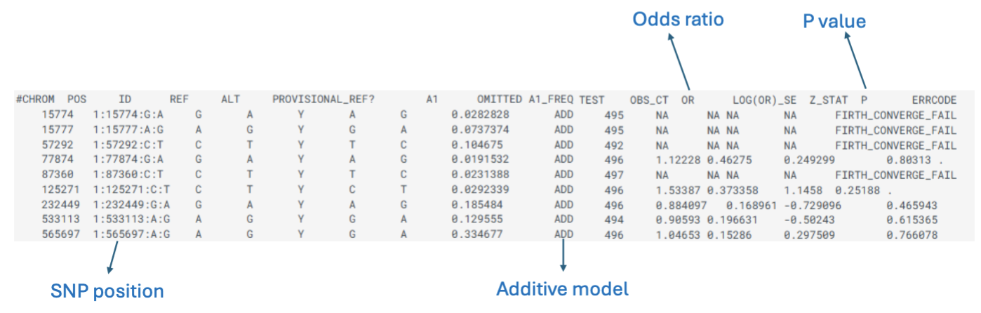
GWAS example

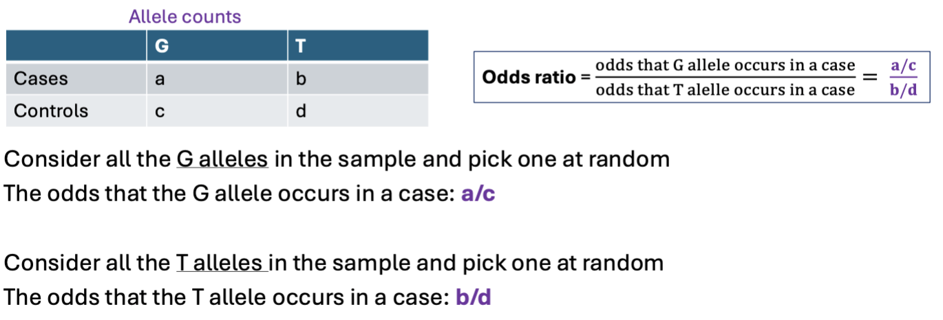
Odds ratio

• Measure of effect size.

• OR = 1, no disease association.

• OR > 1, allele C increases risk of disease.

• OR < 1, allele C decreases the risk of disease.

PLINK

• A software tool for analyzing genetic data, especially for GWAS, including association testing, quality control, and data management.

• Mostly shared.

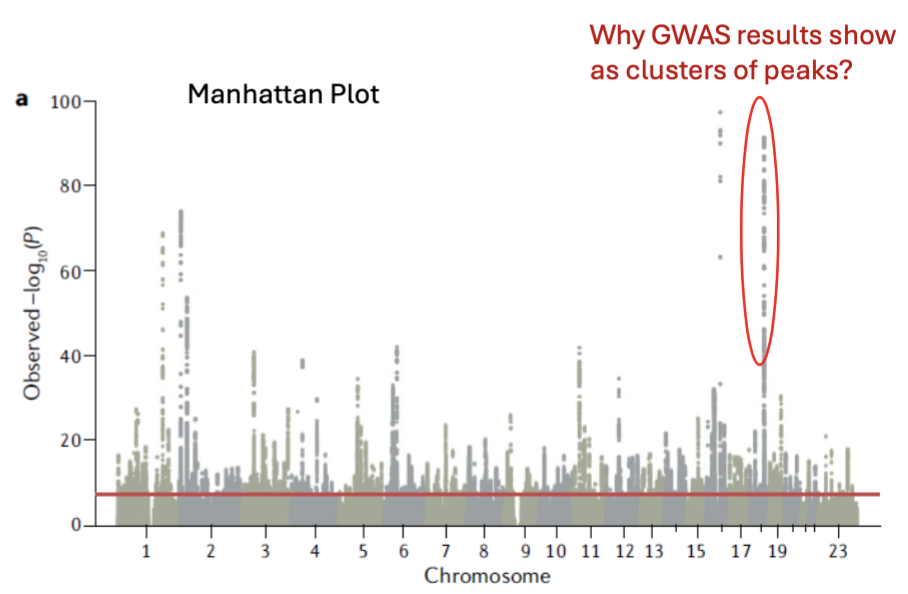
How do we visualize GWAS results

• Manhattan plot:

  • Bonferroni testing threshold of p < 5 × 10^-8.

    • Multiple test correction.

  • Genome-wide significance threshold = red line on the image.

    • The peaks are SNPs that are close to each other = co-inherited.

  • Significance threshold varies depending on:

    • Number of SNPs examined.

    • Number of subjects included.

    • Minor allele frequencies.

    • Etc.

• LocusZoom: a combination of a Manhattan plot and a genome browser.

Genotype datasets for large scale GWAS

• Biobanks and large population-based studies with genetic and phenotype data available for research.

  • For USA → ‘All of Us’ initiative or 23andMe.

• Genotype data are typically restricted due to re-identification risk.

  • Application needed.

Databases for GWAS summary statistics

• GWAS Catalog.

• GWAS Atlas.

• Allow easy access to summary statistics for thousands of traits.

• Many downstream analyses are built on the summary statistics, rather than the raw genotype itself.

Post-GWAS analysis

• Functional mapping:

  • Where are they located in the DNA?

  • Pathways enriched by GWAS findings.

  • How may they influence molecular functions leading to disease?

  • Identify the tissues or cell types where these variants are likely to act.

• Causal variants identification:

  • GWAS findings come up as clusters → highly correlated.

  • Which one is likely causal?

• Polygenic risk score.

Functional mapping of GWAS findings - Where are they located in the DNA?

• Chromosome & base pair position.

• Coding regions: synonymous / nonsynonymous.

• Non-coding regions (majority): introns, promoters, enhancers, histone marks, DHS sites.

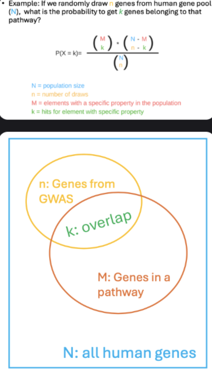
• Pathway analysis: link nearest genes to biological pathways; test overlap significance with hypergeometric test (e.g., via EnrichR).

Functional mapping of GWAS findings - How may they influence molecular functions leading to disease?

• eQTL: SNP affecting gene expression.

  • Other QTLs: pQTL, methylation QTL, etc.

• Link DNA → gene expression → molecular/phenotypic traits → disease risk.

Functional mapping of GWAS findings - Which tissues or cell types these variants are likely ot act on?

• GWAS SNPs: eQTLs are tissue- and/or cell-specific.

• Nearest genes of GWAS SNPs.

GTEx project

• Studies how genetic variation affects gene expression in normal human tissues.

• Focuses on nearby (cis) eQTLs.

• eGene: gene whose expression is significantly influenced by ≥1 nearby eQTL.

Functional mapping of GWAS findings - Causal variants identification

• Fine-mapping is a statistical analysis that identifies the causal variant(s) within a GWAS locus for a disease.

• CausalDB.

Fine mapping steps

1. Define locus: pick region of interest from GWAS.

2. Expand region: include variants in LD with lead SNP.

3. Gather data: association stats (z-scores/SE), LD info.

4. Identify causal variants: heuristic LD, penalized regression, Bayesian models.

Heuristic LD approach

• Pick the lead SNP + group nearby correlated SNPs based on LD thresholds.

• High LD = inherited together.

Penalized linear regression approach

• Penalize the regression to avoid overfitting when SNPs are numerous and correlated.

• Only a few SNPs within a region are causal.

Bayesian models

• Posterior inclusive probability (PIP): probability a SNP is causal given data/model.

• Credible set: variants whose cumulative PIP reaches confidence threshold (e.g., 95%).

• Goal: make credible set as small as possible.

• Tools: CAVIAR, FINEMAP, SuSiE, PAINTOR.

Heritability

• Measures how much of the variation in a trait is due to genetic differences.

• A heritability of 0.7 means that genetic factors explain 70% of the variation in that trait.

• Can either be:

  • Twin-based:

    • Gold standard for estimating the broad-sense heritability.

  • GWAS-based.

  • SNP-based.

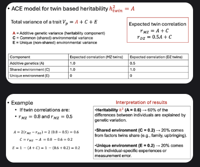
Twin-based heritability

• Compare similarity of traits in relatives.

• Closer relatives share more genes: MZ (monozygotic) twins ~100%, DZ (dizygotic) twins ~50%.

• If MZ similarity ≫ DZ similarity → trait largely genetic.

ACE model for twin based heritability

GWAS-based heritability

• Definition: proportion of trait variance explained by genotyped SNPs.

• From genotype data: use GRM (Genetic Relationship Matrix) → tool: GCTA.

  • GRM is based on pairwise genetic similarities between individuals.

• From GWAS summary stats: regress SNP test stats (χ²) on LD scores → tool: LDSC.

Missing heritability

• Definition: portion of trait variance not captured by GWAS.

• Due to: rare variants (mendelian variants), structural variants, small-effect common SNPs (polygenic risk scores).

Genome-wide Complex Trait Analysis (GCTA)

• Estimates heritability explained by all common SNPs simultaneously.

• Finds that common SNPs collectively explain a substantial portion of trait heritability.

• Explains more than GWAS hits but less than twin-based estimates.

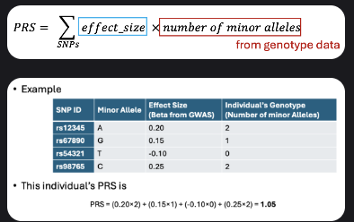
Polygenic risk score

• Definition: summarizes overall genetic risk for a trait/disease in a single value.

• Combines effects of many variants; each contributes a small amount.

• Metrics: association (p-value), variance explained (R²), effect size (β/OR), discrimination (AUC).

• Tools: LDPred, PRSice.

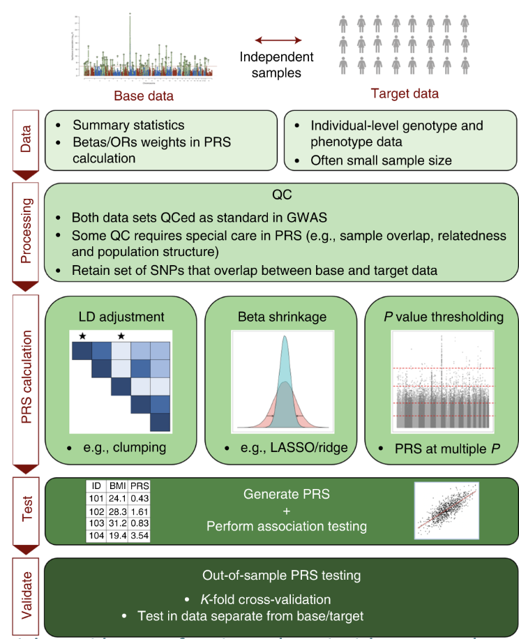
Fundamental steps of a PRS analysis

• Base & target QC: check GWAS heritability, different populations, allele alignment, sample size, genome build.

• PRS calculation: control for LD, adjust for inflated GWAS effect sizes.

• PRS testing & validation.

Interpreting PSR

• Can convert PRS to z-scores or percentiles for comparison.

• Top decile → higher disease risk vs. bottom decile.

• Probabilistic: high PRS ≠ guaranteed disease, low PRS ≠ protection.

PSR applications

• Applications: patient stratification (grouping patients based on risk), prevention, trials.

• Limits: partial heritability, ancestry bias, ignores interactions (gene-gene interactions), GWAS-dependent (power depends on GWAS sample size and quality).