Looks like no one added any tags here yet for you.
What is timing-based reconstruction in imaging?
Timing-based reconstruction involves using timing information in a signal to determine positions within the body.
- Typically applies to reflection-based methods like ultrasound imaging.
- Relies on sending pulses of ultrasound and analyzing the timing of returned echoes to infer depth.
How does ultrasound imaging work for timing-based reconstruction?
- Ultrasound pulses are transmitted into the body.
- Reflected waves (echoes) from interfaces are detected.
- Deeper interfaces reflect waves that take longer to return compared to nearer ones.
- This timing difference helps infer depth in the received signal.
What is the difference between continuous-wave and pulsed ultrasound?
- Continuous-wave ultrasound: Useful for Doppler measurements but lacks the ability to localize reflections.
- Pulsed ultrasound: Enables localization of reflections and depth inference, crucial for imaging.
What is A-Mode imaging?
- A-Mode (Amplitude Mode) imaging generates a one-dimensional plot of received intensity versus time.
- Assumes a uniform speed of sound to convert timing of echoes into depth.
- Represents the simplest form of ultrasound imaging, displaying depths of interfaces along a single beam line.
What is a limitation of A-Mode imaging?
A-Mode imaging neglects the effect of attenuation, causing echoes from deeper interfaces to have smaller amplitudes compared to those from nearer interfaces.
How can attenuation in A-Mode imaging be corrected?
Time gain compensation (TGC) is used to amplify pulses in proportion to their depth.
- The measured signal amplitude is multiplied by the inverse of the attenuation equation.
- Requires information about the depth of the interface and assumes a uniform speed of sound.
What are the assumptions and limitations of time gain compensation (TGC)?
- Assumes a uniform attenuation coefficient, which is an oversimplification.
- Does not account for detailed effects of transmission and reception by the transducer in a pulse-echo system.
What is Time Gain Compensation (TGC), and how is it used in ultrasound imaging?
Time Gain Compensation (TGC) is a method used in ultrasound imaging to correct for the attenuation of sound waves as they travel through tissue. Attenuation causes the amplitude of reflected signals to decrease with depth, making it harder to detect echoes from deeper structures.
To compensate for this, the received signal is multiplied by a factor TGC(t) , which increases over time (corresponding to deeper regions). The factor is given by:
TGC(t) = e^{\mu c t}
where:
- \mu : Attenuation coefficient.
- c : Speed of sound in the medium.
- t : Time since the pulse was launched.
This ensures that echoes from deeper scatterers are amplified appropriately to match those from shallower depths, improving image uniformity and diagnostic accuracy.
What is Exercise 7A about? How can you determine the depth of interfaces and calculate TGC?
Exercise 7A involves calculating the depth of ultrasound interfaces based on echo timings and compensating for attenuation using Time Gain Compensation (TGC). Here's how:
Part (a): Calculating the depth of interfaces
1. Use the formula for distance:
\text{Distance} = \text{Speed} \times \text{Time}
However, ultrasound travels "there and back," so divide the total distance by 2.
2. Speed of sound in tissue = 1540 \, \text{m/s}.
3. Echo timings:
- For the 1.3 µs echo:
\text{Distance} = 1540 \, \text{m/s} \times 1.3 \times 10^{-6} \, \text{s} = 0.002 \, \text{m (2 cm total)}.
Depth = 1 \, \text{cm}.
- For the 6.5 µs echo:
\text{Distance} = 1540 \, \text{m/s} \times 6.5 \times 10^{-6} \, \text{s} = 0.01 \, \text{m (10 cm total)}.
Depth = 5 \, \text{cm}.
Part (b): Deriving the TGC formula
1. Attenuation is modeled as:
I(x) = I_0 e^{-\mu x}
Where:
- I(x): Attenuated intensity.
- I_0: Initial intensity.
- \mu: Attenuation coefficient.
- x: Distance.
2. To compensate for attenuation, apply:
\text{TGC}(t) = \frac{I_0}{I(x)} = e^{\mu c t}
Where:
- c: Speed of sound in tissue.
- t: Time.
Part (c): TGC Calculations
Step 1: Determine \mu:
Given \mu = 0.87 \, \text{dB/cm} \, \text{MHz}^{-1.5}:
1. For 2.5 \, \text{MHz}:
\mu = 0.87 \times (2.5)^{1.5} = 3.439 \, \text{dB/cm}.
Convert to \text{cm}^{-1}:
\mu = 0.792 \, \text{cm}^{-1}.
2. For 5 \, \text{MHz}:
\mu = 0.87 \times (5)^{1.5} = 9.73 \, \text{dB/cm}.
Convert to \text{cm}^{-1}:
\mu = 2.24 \, \text{cm}^{-1}.
Step 2: Calculate TGC for each echo
1. At 2.5 \, \text{MHz}:
- For the 1.3 µs echo (1 \, \text{cm}):
\text{TGC} = e^{\mu c t} = e^{0.792 \times 1540 \times 1.3 \times 10^{-6}} \approx 4.87.
- For the 6.5 µs echo (5 \, \text{cm}):
\text{TGC} = e^{\mu c t} = e^{0.792 \times 1540 \times 6.5 \times 10^{-6}} \approx 2750.
2. At 5 \, \text{MHz}:
- For the 1.3 µs echo:
\text{TGC} = e^{2.24 \times 1540 \times 1.3 \times 10^{-6}} \approx 88.2.
- For the 6.5 µs echo:
\text{TGC} = e^{2.24 \times 1540 \times 6.5 \times 10^{-6}} \approx 5.35 \times 10^{9}.
Insights
- Higher ultrasound frequencies result in greater attenuation, requiring higher TGC to compensate.
- However, higher frequencies improve spatial resolution, balancing depth penetration and detail.
What is axial resolution?
Axial resolution is the ability of an imaging system, such as ultrasound, to distinguish between two objects that are close together along the depth axis (the direction of the ultrasound beam). It is determined by the pulse duration and the speed of sound in the medium. A shorter pulse duration improves axial resolution, allowing for better separation of closely spaced objects.
What determines the axial resolution in an ultrasound image?
Axial resolution is determined by the pulse duration p_d , as it depends on distinguishing echoes from interfaces that overlap by at most half their duration:
\text{Axial resolution} = \frac{1}{2} p_d c
Where c is the speed of sound in tissue. This is half the length of a pulse.
Imagine a pulse being a really long train. As the trains reflect, there is a chance one train overlaps another. This happens when the reflection of one pulse hasn’t fully ended and the reflection of another pulse has come and begun to overlap.
Axial resolution refers to the minimum distance between two objects along the direction of the ultrasound beam (depth axis) that the system can distinguish as separate objects.
Imagining pulses as long trains, the smallest gap between two interfaces can be half the length of a train. This can be visualised if you try hard enough…
What happens if A-mode scanning is repeated line-by-line?
Repeating the A-mode scan line-by-line produces an M-mode "image," useful for observing highly mobile tissues like the heart.
What are the characteristics of the ultrasound beam in pulse-echo imaging?
1. The sound beam spreads out conically from the transducer, unlike the simplified model where sound travels strictly perpendicular.
2. Reflected echoes return to the transducer from a volume of tissue, across a range of angles.
How can the pulse be modeled in ultrasound?
The pulse n(t) can be modeled as:
n(t) = n_e(t) e^{-j(2\pi f_0 t - \phi)}
Where:
- n_e(t) : Envelope representing the shape of the pulse. It determines the amplitude.
- f_0 : Ultrasound frequency.
- \phi : Arbitrary phase offset.
- Each transducer point acts as an acoustic dipole. This means each point of the transducer is treated as producing waves.
What is the pressure at a point due to contributions from a flat transducer?
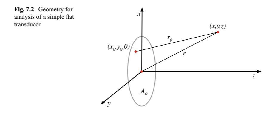
The total acoustic pressure p(x, y, z, t) at a point is the sum of contributions from all points on the transducer's surface A_0 :
p(x, y, z, t) = \int_{}\int_{A_0} \frac{z}{r_0^2} n\left(t - \frac{r_0}{c}\right) dx_0 dy_0
Where:
- r_0 = \sqrt{(x - x_0)^2 + (y - y_0)^2 + z^2} : distance from a point (x_0, y_0) on the transducer to the observation point.
- n(t) : shape of the emitted acoustic pulse.
- z : perpendicular distance of the observation point from the transducer.
Note: x,y,z is always a scatter point in space, and x_0, y_0, z_0 is a point on transducer.
How is the scattered intensity contribution modeled?
For scattering from a location (x, y, z) , the scattered pressure contribution p_s(x_0', y_0', t) at a point (x_0', y_0', 0) [the zero referring to z = 0] on the transducer face is:
p_s(x_0', y_0', t) = \int_{}\int_{A_0} R(x, y, z) \frac{z}{r_0'^2} p\left(x, y, z, t - \frac{r_0'}{c}\right) dx_0' dy_0'
Where:
- r_0' = \sqrt{(x - x_0')^2 + (y - y_0')^2 + z^2} : distance from the scattering point to the point (x_0', y_0', 0) on the transducer.
- R(x, y, z) : scattering intensity as a function of position.
- p(x, y, z, t) : pressure at the scattering point.
Each point on the transducer's surface acts as a source of sound waves (like tiny acoustic dipoles).
Emit a pulse toward a scattering point in the medium.
That pulse is scattered by the tissue at that point.
The scattered wave travels back to the transducer.
Equation integrates over the whole transducer surface to capture the received pressure. By choosing a specific value of (x_0', y_0', 0) , we can get the value for the pressure at that point.
How is the final scattered pressure expression p_s(x_0', y_0', t) derived, starting from its integral?
The final scattered pressure expression is derived by substituting the pressure equation p(x, y, z, t) into the original integral. Here’s the process:
1. Original Integral for Scattered Pressure (for whole pulse journey):
p_s(x_0', y_0', t) = \int \int_{A_0} R(x, y, z) \frac{z}{r_0'^2} p(x, y, z, t - c^{-1}r_0') dx_0 dy_0
- R(x, y, z) : Scattering function.
- \frac{z}{r_0'^2} : Depth and geometric spreading term.
- p(x, y, z, t - c^{-1}r_0') : Pressure at the scattering point delayed by the time for the wave to return to the transducer.
2. Pressure Expression at a Point ( p(x, y, z, t) ) (from transducer to point):
Substitute p(x, y, z, t) from Equation (7.4):
p(x, y, z, t) = \int \int_{A_0} \frac{z}{r_0^2} n\left(t - c^{-1}r_0\right) dx_0 dy_0
3. Substitution into the Scattered Pressure Equation:
Replace p(x, y, z, t) in the original integral:
p_s(x_0', y_0', t) = \int \int_{A_0} R(x, y, z) \frac{z}{r_0'^2} \left( \int \int_{A_0} \frac{z}{r_0^2} n\left(t - \frac{r_0}{c} - \frac{r_0'}{c}\right) dx_0 dy_0 \right) dx_0' dy_0'
- This combines the scattering contribution ( R(x, y, z) ) with the emitted pressure at the scattering point.
4. Resulting Final Equation:
After substitution and simplifying:
p_s(x_0', y_0', t) = \int \int_{A_0} \int \int_{A_0} R(x, y, z) \frac{z}{r_0'^2 r_0^2} n\left(t - \frac{r_0}{c} - \frac{r_0'}{c}\right) dx_0 dy_0 dx’_0 dy’_0
- This accounts for the propagation from the transducer to the scatterer ( r_0 ) and back ( r_0' ).
How is the final scattered pressure expression written?
Combining scattering contributions with the acoustic dipole pattern leads to:
p_s(x_0', y_0', t) = \int \int_{A_0} \int \int_{A_0} R(x, y, z) \frac{z}{r_0'^2 r_0^2} n\left(t - \frac{r_0}{c} - \frac{r_0'}{c}\right) dx_0 dy_0 dx’_0 dy’_0
Where:
- r_0' : distance from the scattering point back to (x_0', y_0') on the transducer.
(substitutes equation for pressure at point x,y,z)
What is the plane wave approximation?
The plane wave approximation assumes that the envelope of the pulse arrives at all points in a given z-plane simultaneously, simplifying the wave behavior and analysis.
How is n(t) approximated under the plane wave approximation?
The pulse n(t) is modeled as:
n(t) = n_e(t) e^{-j(2\pi f_0 t - \phi)}
Under the plane wave approximation, n(t) when arriving at the transducer is expressed as:
n(t) \approx n_e\left(t - 2c^{-1}z\right)e^{-j\left(2\pi f_0(t - c^{-1}r_0 - c^{-1}r_0') - \phi\right)}
or approximately:
n(t) \approx n\left(t - 2c^{-1}z\right)e^{jk(r_0 - z)}e^{jk(r_0' - z)}
where:
- n_e(t) : The envelope of the pulse.
- f_0 : The pulse frequency.
- r_0 and r_0' : Distances between the scatterer and the transducer.
- \phi : Phase shift.
- k : Wave number.
How is the received intensity from a single scatterer expressed?
The received intensity from a single scatterer is written as:
r(x, y, z, t) = K R(x, y, z) n\left(t - 2c^{-1}z\right) q(x, y, z)^2
where:
- K : Gain factor related to the sensitivity of the transducer and receive electronics.
- R(x, y, z) : Scattering function at the point.
- n\left(t - 2c^{-1}z\right) : The time-delayed signal.
- q(x, y, z) : Field pattern for the transducer.
This is the intensity received at the transducer from a specific scatter point, similar to the equation below:
p_s(x_0', y_0', t) = \int \int_{A_0} \int \int_{A_0} R(x, y, z) \frac{z}{r_0'^2 r_0^2} n\left(t - \frac{r_0}{c} - \frac{r_0'}{c}\right) dx_0 dy_0 dx’_0 dy’_0
By assuming the assumption, we develop a simpler equation where the surface integral goes to q, which describes the pattern of intensities meeting the transducer.
How is the field pattern q(x, y, z) defined?
The field pattern q(x, y, z) is defined as:
q(x, y, z) = \int \int_{A_0} \frac{z}{r_0^2} e^{jk(r_0 - z)} dx_0 dy_0
where:
- A_0 : The aperture area of the transducer.
- r_0 : Distance from the transducer to the scatterer.
- k : Wave number.
How is the total signal received from a distribution of scatterers expressed?
The total signal received from a distribution of scatterers is:
r(t) = \int_{0}^\infty \int_{-\infty}^\infty \int_{-\infty}^\infty K R(x, y, z) n\left(t - 2c^{-1}z\right) e^{-2\mu z} q(x, y, z)^2 dx dy dz
where:
- e^{-2\mu z} : Attenuation factor.
- \mu : Attenuation coefficient.
- Other terms are as defined previously.
How is the total signal received from a distribution of scatterers expressed?
The total signal received from a distribution of scatterers is expressed as:
r(t) = \int_{0}^\infty \int_{-\infty}^\infty \int_{-\infty}^\infty K R(x, y, z) n\left(t - 2c^{-1}z\right) e^{-2\mu z} q(x, y, z)^2 dx dy dz
where:
- K : Gain factor related to the transducer sensitivity.
- R(x, y, z) : Scattering function at each point.
- n(t - 2c^{-1}z) : Time-delayed signal.
- q(x, y, z) : Field pattern of the transducer.
- e^{-2\mu z} : Attenuation factor incorporating the attenuation coefficient \mu .
What does the new integral representation of r(t) indicate, and how does \tilde{q}(x, y, z) differ from q(x, y, z) ?
The integral for the received signal r(t) can be rewritten as:
r(t) = K' \frac{e^{-\mu ct}}{(ct)^2} \int_0^\infty \int_{-\infty}^\infty \int_{-\infty}^\infty R(x, y, z) n\left(t - 2c^{-1}z\right) \tilde{q}(x, y, z)^2 dx dy dz,
where:
- \tilde{q}(x, y, z) = z q(x, y, z) is a modified form of q(x, y, z) , which scales the field pattern q(x, y, z) by the scatterer depth z .
- q(x, y, z) originally represents the field pattern contribution at the scatterer, accounting for the transducer geometry and wave interference.
- By defining \tilde{q}(x, y, z) , the z -dependency is explicitly factored out, making it easier to isolate the scatterer’s depth in the final expression.
What does the Time Gain Compensation (TGC) and the corrected received signal integral represent?
To correct for attenuation in the received signal, Time Gain Compensation (TGC) is applied. The form of TGC suggested is:
TGC(t) \propto (ct)^2 e^{\mu ct},
where:
- (ct)^2 : Accounts for geometric spreading.
- e^{\mu ct} : Compensates for exponential attenuation due to tissue absorption.
Corrected Received Signal Integral
The corrected signal r_c(t) after applying TGC is given by:
r_c(t) = \int_{0}^\infty \int_{-\infty}^\infty \int_{-\infty}^\infty R(x, y, z) n_e(t - 2c^{-1}z) e^{j(2\pi f_0 (t - 2c^{-1}z) - \phi)} \tilde{q}(x, y, z)^2 dx dy dz,
where:
- n_e(t) : Represents the envelope of the emitted pulse.
- \tilde{q}(x, y, z) : Modified field pattern scaled by scatterer depth z .
- R(x, y, z) : Scattering intensity.
Purpose of the Correction
1. TGC Application: Ensures that attenuation and geometric spreading are compensated, allowing a more accurate representation of the received signal.
2. Corrected Integral: Models the received signal with compensation applied, incorporating both amplitude corrections and phase components.
What is the form of the received signal, and what does it represent?
The received signal r_c(t) is written as:
r_c(t) = r_e(t) e^{-j(2\pi f_0 - \phi)},
where r_e(t) is the envelope of the signal, which carries information about the amplitude, and e^{-j(2\pi f_0 - \phi)} is the carrier wave at frequency f_0 . The envelope r_e(t) can be separated from the carrier using demodulation techniques and depends on the scattering strength R(x, y, z) . However, other factors, like the field pattern q(x, y, z) , also affect the signal, making the amplitude more complex to interpret.
How does the field pattern and transducer design affect imaging?
The field pattern q(x, y, z) plays an important role in shaping the signal and the resulting image. It represents how the transducer directs ultrasound energy and captures reflections. To improve imaging, curved transducers or transducer arrays are often used. These setups create more focused beams, which help capture clearer images, and allow for steering the ultrasound beam to explore different regions without moving the transducer.