H8: Multi-Agent RL (MARL) - deel 1

Wat is MARL

• Multi-agent reinforcement learning (MARL) is about finding optimal decision policies for two or more artificial agents interacting in a shared environment

• applying RL algorithms to multi-agent systems

• goal is to learn optimal policies for two or more agents

MARL for solving multi-agent systems

• lockstep?

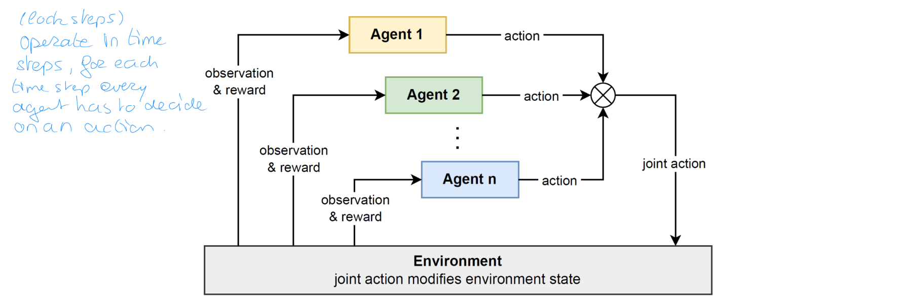
• Goal: learn optimal policies for a set of agents in a multi-agent system

• Each agent chooses an action based on its policy => joint action

• Joint action affects environment state; agents get rewards + new observations

Lockstep: operate in timesteps, for each timestep every agent has to decide on an action

Why should we use MARL to find optimal solutions to multi-agent systems rather than controlling multiple 'agents' using a single-agent RL (SARL) algorithm?

• Decomposing a large problem

  • In LBF example, controlling 3 robots each with 6 actions, the joint actoin space becomes 6³ = 216 (huge)
    -> large action space for SARL

  • We can decompose this into three independent agents, each selecting from only 6 actions
    -> use MARL to train seperate agent policies (more tractable)

• Decentralized decision making

  • 1 policy on every agent

  • There are many real world scenarios where it is required for each agent to make decisions independently

  • e.g. autonomous driving is impractical for frequent long-distance data exchanges between a central agent and the vehicle

Challenges of MARL(4)

• non-stationarity caused by multiple learning agents

  • if multiple agents are learning, the environment becomes non-stationary from the perspective of individual agents

  • => moving target: each agent is optimizing against changing policies of other agents

  • Multiple stable solutions are possible in more complex environments. Agents need to negotiate which solution they converge to.

• Optimality of policies and equilibrium selection

• multi-agent credit assignment

  • Which agents actions contributed to received rewards

  • voorbeeld van appels oppakken

    • At time step t all agents perform collect, each receiving reward + 1

    • Whose actions led to the reward

    • the agent on the left did not contribute

    • Learning agents must disentangle the contributions of actions

• Scaling in number of agents

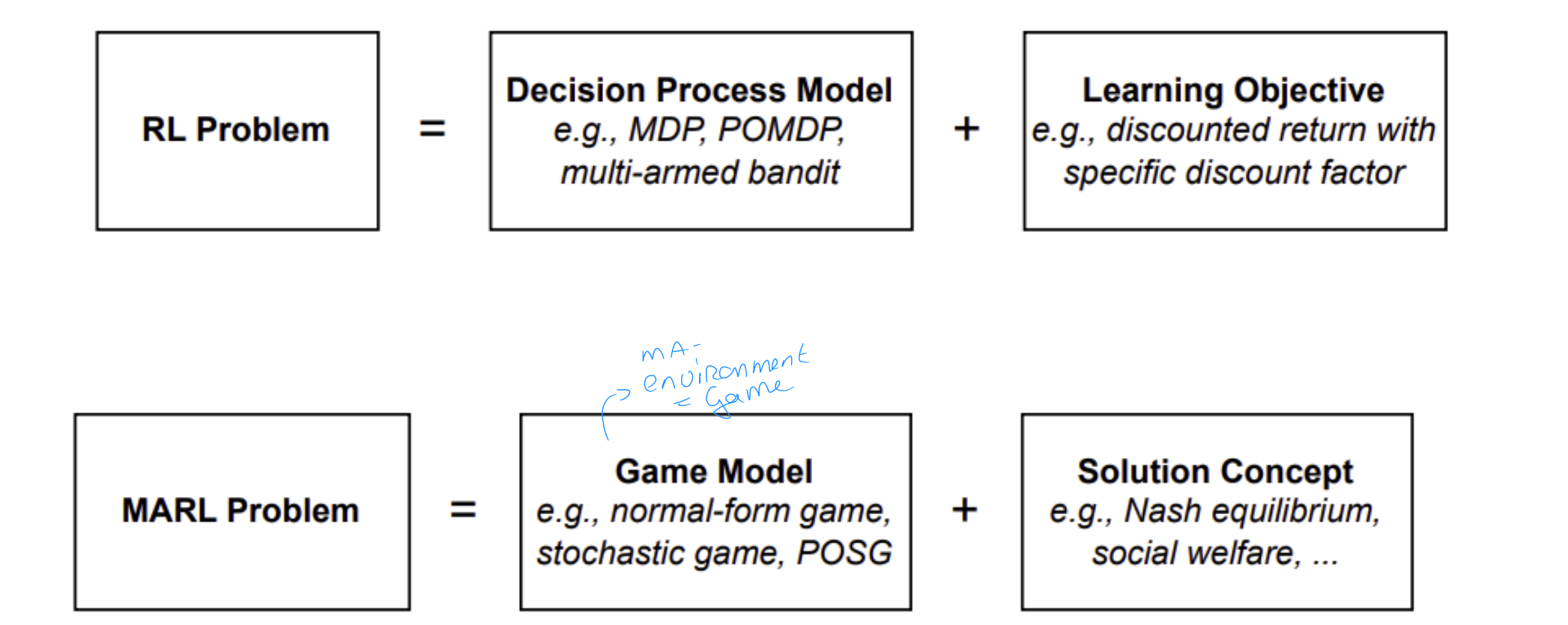
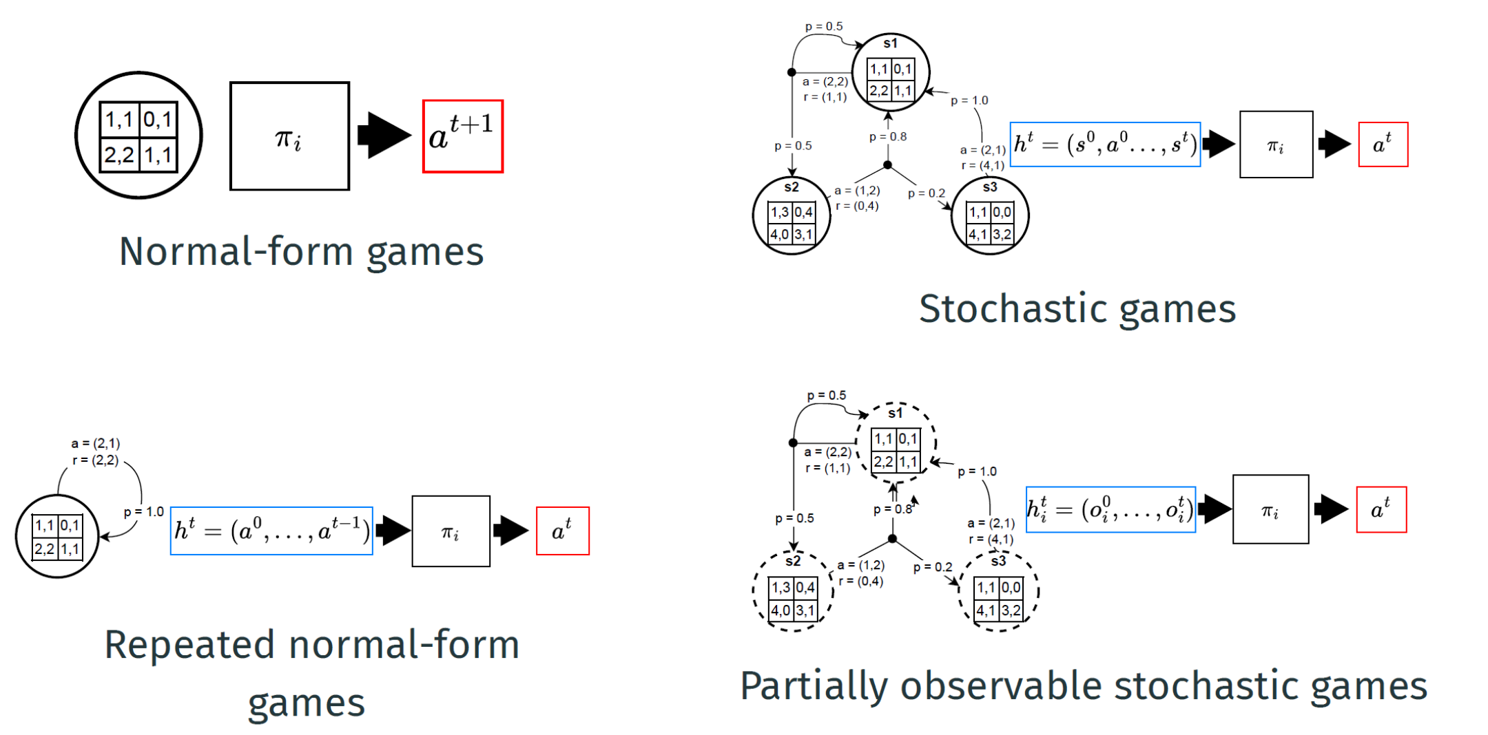
Components of RL problem vs MARL problem

Normal-form games

Normal-form games define a single interaction between two or more agents, providing a simple kernel for more general games to build upon.

Normal-form games are defined as a 3 tuple (I,{Ai​}i∈I, {Ri}i∈I):

• I is a finite set of agents I = {1,.., n}

• For each agent i∈I

  • Ai is a finite set of actions

  • Ri​ is the reward function Ri:A→R where A=A1×..×An (set of joint actions)

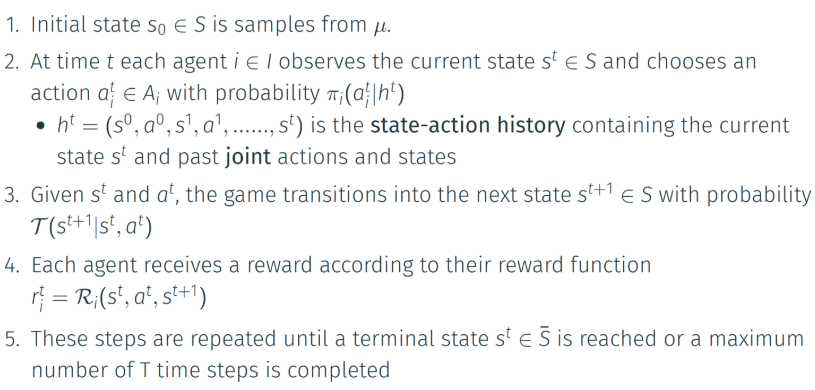
Normal-Form game process

In a normal-form game, there are no time steps or states. Agents choose an action and observe a reward.

The game proceeds as follows:

1. Each agent samples an action ai∈Ai with probability πi(ai)

2. The resulting actions from all agents form a joint action, a = (a1,...,an​)

3. Each agent receives a reward based on its individual reward function and the joint action, ri=Ri(a)

Classes of games

Games can be classified on the relationship between the agents reward functions.

• In zero-sum games, the sum of the agents reward is always 0. Example: ∑i∈IRi(a)=0,∀a∈A

• In common-reward games, all agents receive the same reward (Ri=Rj;∀i,j∈I)

  • example team-game, we all win/lose together

• In general-sum games, there are no restrictions on the relationship between reward functions

Matrix games

• Normal-form games with 2 agents are also called matrix games because they can be represented using reward matrices.

Repeated Normal-Form games

To extend normal-form games to sequential multi-agent interaction, we can repeat the same game over T timesteps

• At each time step t an agent i samples an action aitait​

• the policy is now conditioned on a joint-action history πi(ait∣ht)πi​(ait​∣ht) where ht=(a0,...,at−1)ht=(a0,...,at−1)

• In special cases, htht contains n last joint actions.
  E.g. in a tit-for-tat strategy, the policy is conditioned on at−1at−1

= The multi-agent equivalent of the single-agent multi-armed bandit

Zelfde maar nl:

Hieronder volgen de belangrijkste kenmerken op basis van de bronnen:

• Eén toestand (1 state): In de hiërarchie van games bevinden deze spellen zich op het niveau waar er n agenten zijn, maar de omgeving zelf niet van toestand verandert; het is simpelweg hetzelfde spel dat telkens opnieuw wordt gespeeld.

• Joint-action history (ht): Omdat het spel herhaaldelijk wordt gespeeld, kunnen agenten hun gedrag aanpassen op basis van wat er eerder is gebeurd. De policy van een agent is daarom geconditioneerd op de gezamenlijke actiegeschiedenis, die alle acties van alle spelers uit de voorgaande rondes bevat.

• Conditionele strategieën: Een specifiek voorbeeld dat in de bronnen wordt genoemd, is de tit-for-tat strategie. Hierbij is de actie van een agent direct afhankelijk van de laatst genomen actie van de tegenstander (at−1).

• Leerproces: Bij elke tijdstap t kiest elke agent i een actie (ait​), waarna zij een beloning ontvangen op basis van de gezamenlijk gekozen acties. Dit stelt agenten in staat om complexe interacties zoals samenwerking of vergelding te ontwikkelen over de tijd.

Stochastic games

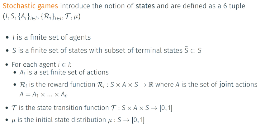
• Each state can be viewed as a non-repeated normal-form game

• stochastic games can also be classified into: zero-sum, common-reward, or general-sum

Stochastic (Markovian) Game process

The stochastic game is a Markov game if the transition distribution is Markovian

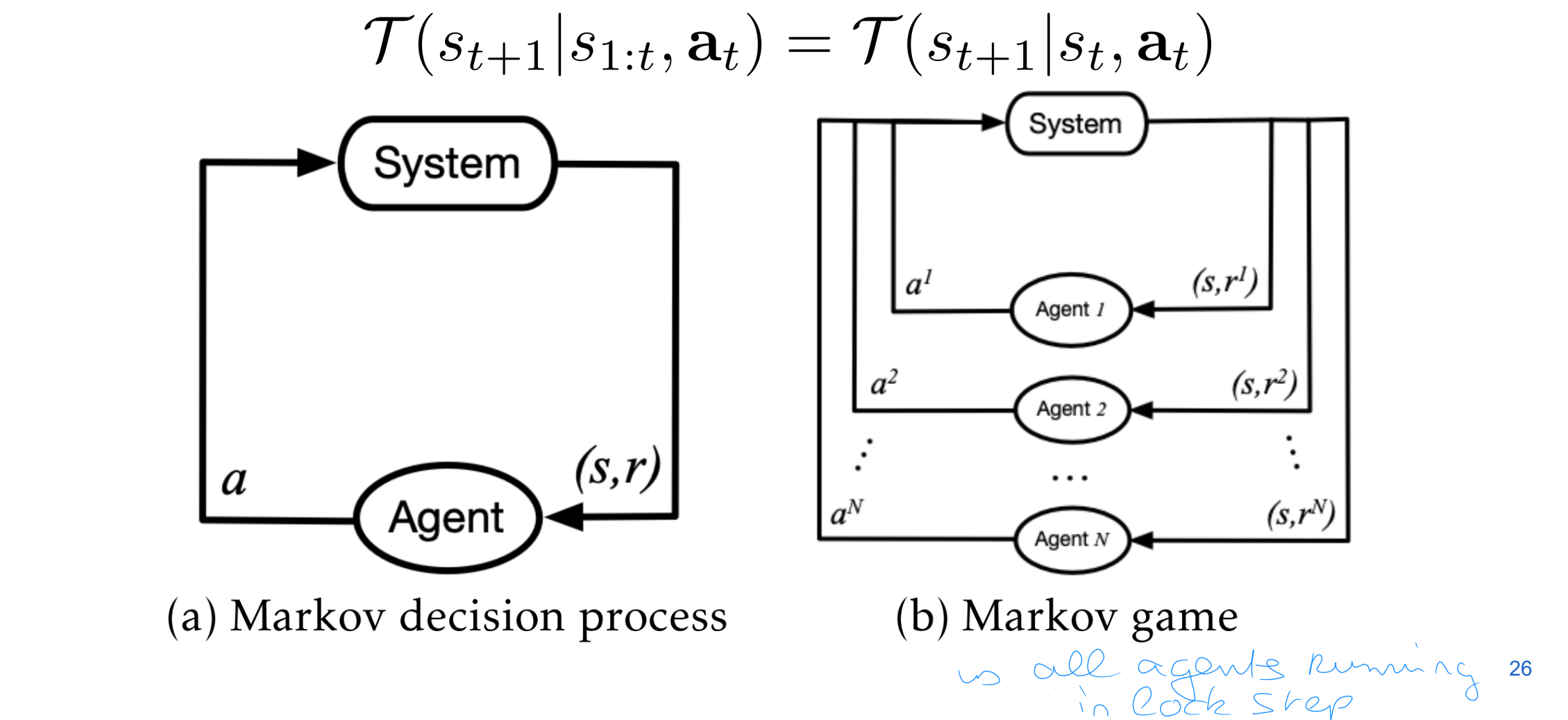
Markov policy

Single agent perspective is non-stationary

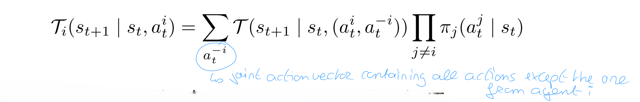
From the perspective of agent i, the environment transition function has the form:

This transition thus depends on the actions of other players

• other agents may be learning -> non-stationarity, even with stationary environment dynamics

• policies of other agents often not known -> must be learned, or treated as source of environment stochasticy

So single agent RL really difficult because env changes constantly

Partially Observable Stochastic games (POSG)

-> most realistic to real life

At the top of the game model hierarchy, the most general model is the POSG

• POSGs represent complex decision processes with incomplete information

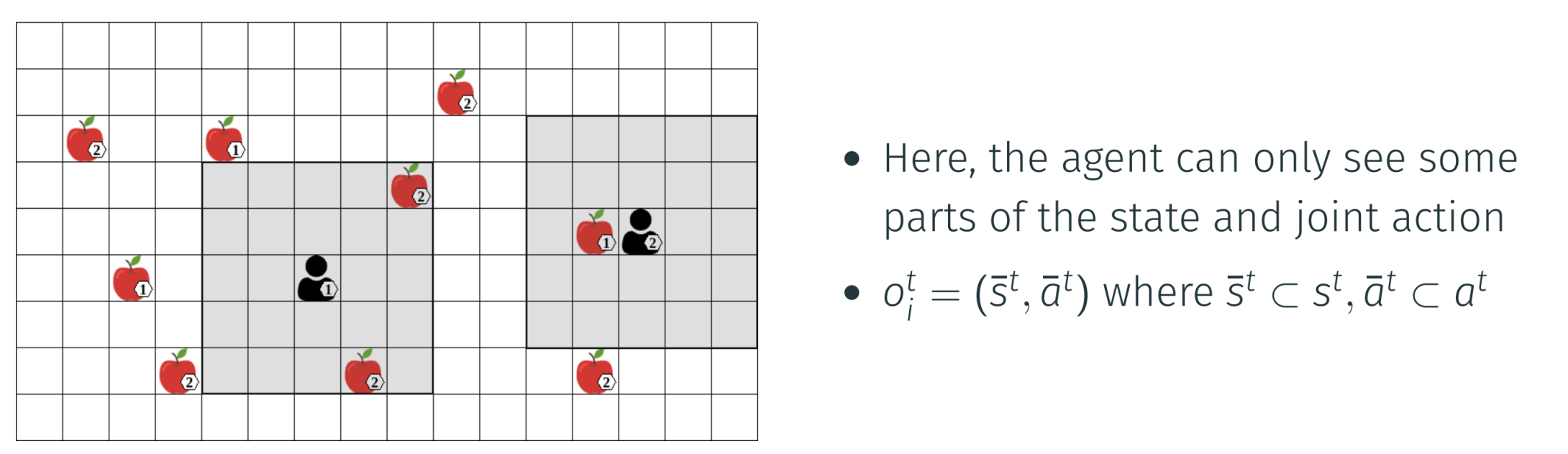
• Unlike in stochastic games, agents receive observations providing incomplete information about the state and agents actions

• POSGs apply to scenarios where agents have limited sensing capabilities
  => e.g. autonomous driving
  => e.g. strategic games with private, hidden information (card games)

Examples of partial observability

• hidden cards in deck or hand of opponent

• limited visibility on map

• simultaneous moves of players

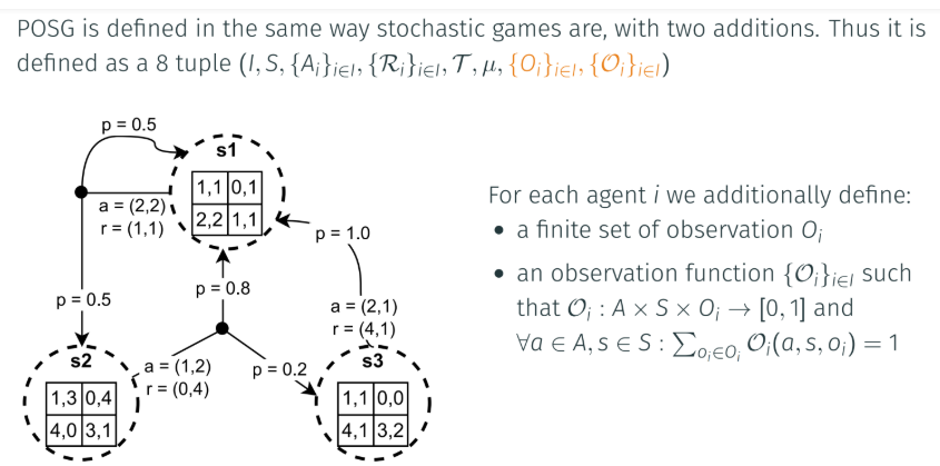
POSG observations

• for each agent, an observation distribution is defined
  

  

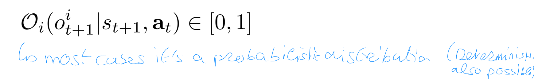
• The environment decides what is included in each observation
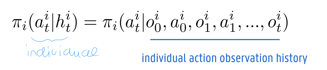
  e.g. it may or may not include the actions of the other agents

• Agent policy has the form:
  

  

The observation function:
POSG can represent diverse observability conditions. For Example:

• Modeling noise by adding uncertainty in the possible observation

• to limit the visibility region of agents (see LBF example)
  

  

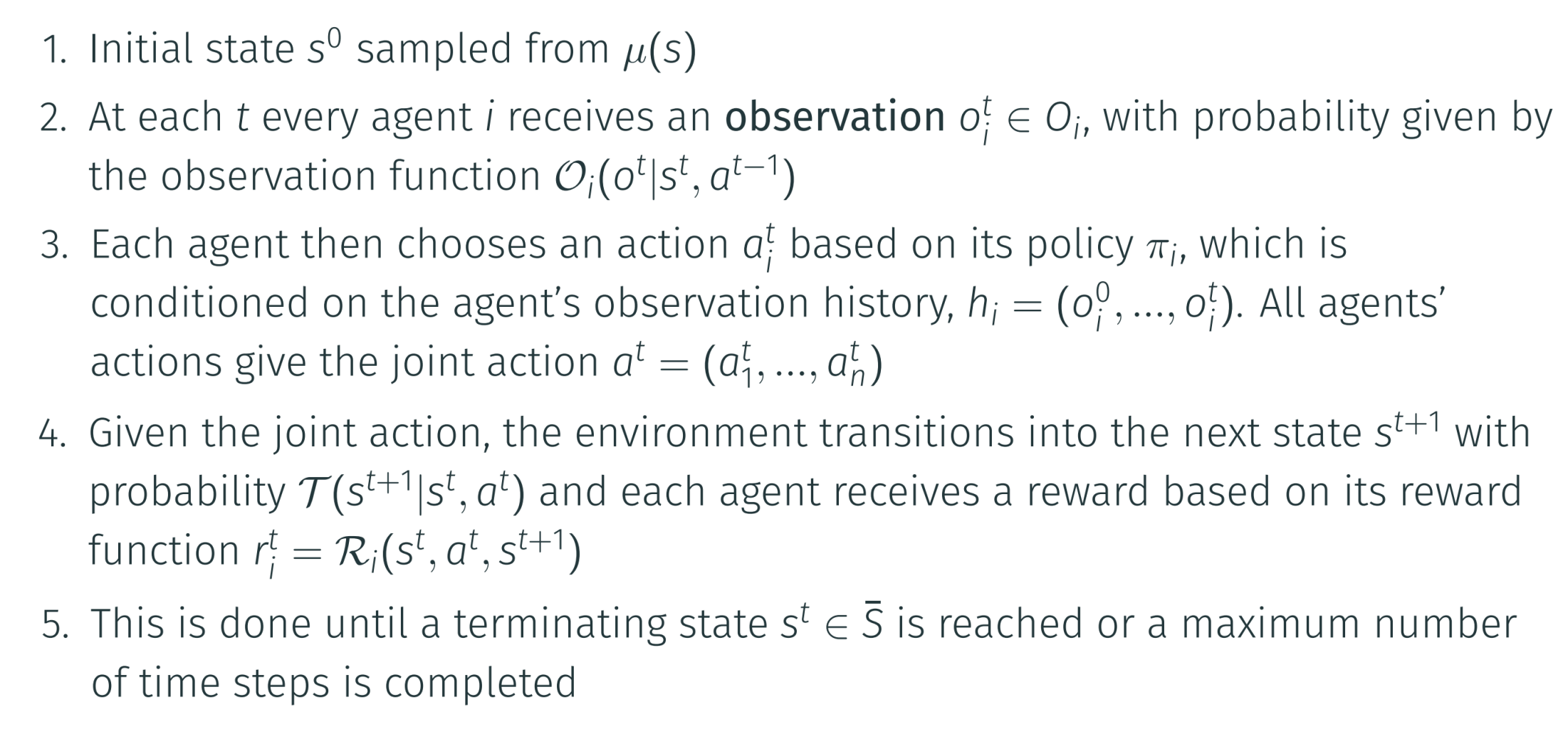
POSG process

belief state

belief state: probability distribution over all possible states the world could be in

In partially observable settings, it becomes more challenging to infer optimal actions. For Example:

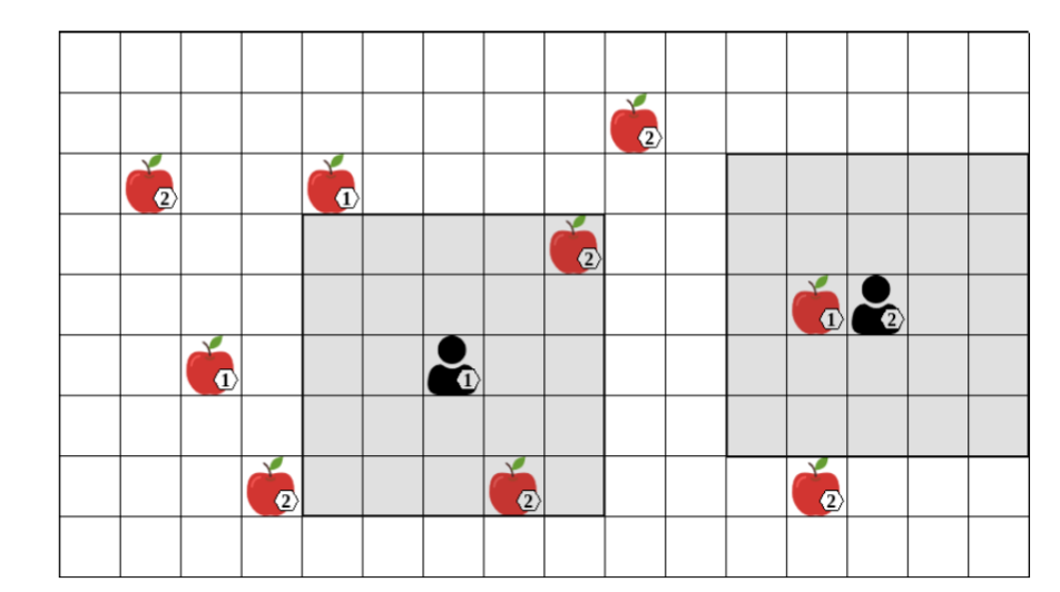
• optimal action for agent 1 is to move left towards level 1 apple

• but level 1 apple is not directly observable

• Agent 1 can hold a belief state b^i_t​, a probability distribution over possible state s ∈S

• Agent 1 might have seen the level-1 apple previously and can thus 'remember' its location

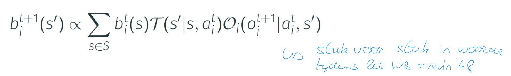
beliefs in single agent settings

To simplify, let's consider the single-agent perspective:

• the initial belief state is given by bi0=μbi0​=μ

• After taking action aitait​ and observing oit+1oit+1​, the belief state bitbit​ is updated to bit+1bit+1​ using a bayesian update:
  

  

In MARL this type of update is typically infeasible:

• High-dimensional state spaces make storage and updates of beliefs intractable

• In MARL for POSG, agents assumed not to know (S, T, speciale OiOi​)

• Deep learning can be used to approximate state information

beliefs in multi-agent settings

The agent observes a sequence of observations generated by the following non-markovian distribution:

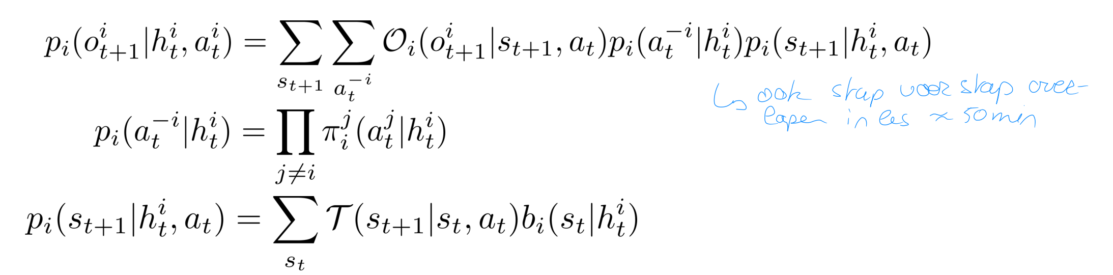
Two options:

• Independent learners

  • Each agents learns form a non-Markovian transition function

  • essentially treating the agents as part of the environment

• Explicitly modelling the other agents

  • requires the agent to estimate the transition function, its local observation model, the observation model of the other agents and of the other agents policies (cheat code CTDE)

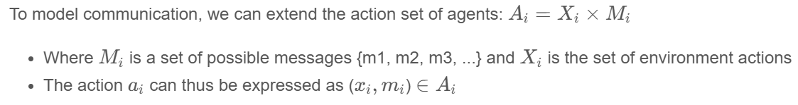
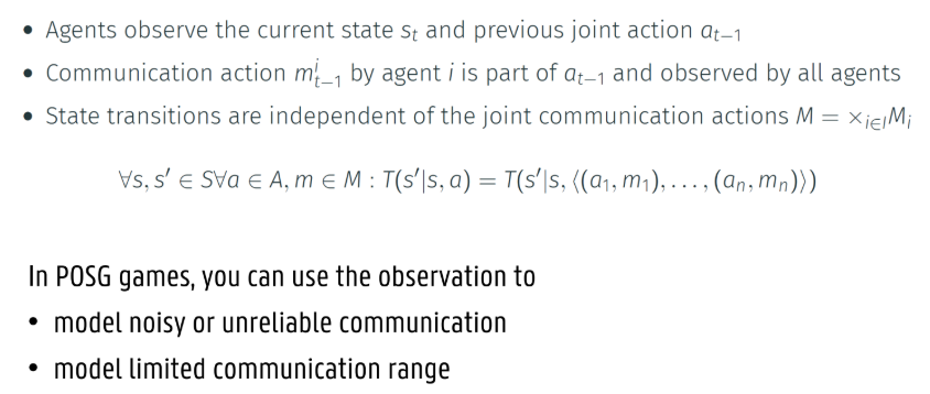
Modeling communication

• using games, we can model more complex agent interactions, such as communication

• We can view communication as a type of action that other agents can observe without affecting the state of the environment

• agents learn communication meanings through trials and observations, identical to environment actions

• this can lead to the evolution of a shared language or protocol

Communication in stochastic games

Solution concepts:

What is an solution in games? What does it mean to act optimally in a multi-agent system?

• Maximizing returns of one agent is no longer enough to determine a solution

• We must consider the joint policy of all agents

• This is less straightforward, and there are many different solution concepts

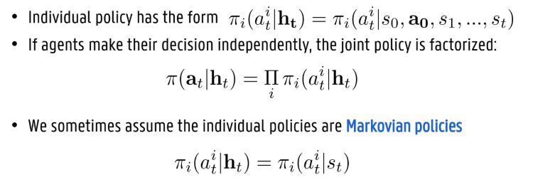
individual policy vs joint policy

Individual policy: inputs of policies depend on game model

The joint policy is the combination of all agents' policies: π=(π1,...,πn)

Probability of a joint action under joint policy πis defined as:

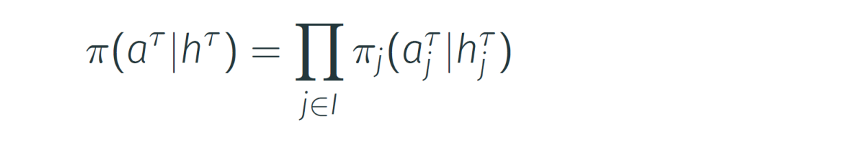
Note: this definition assumes probabilistic independence between agents' policies

notation

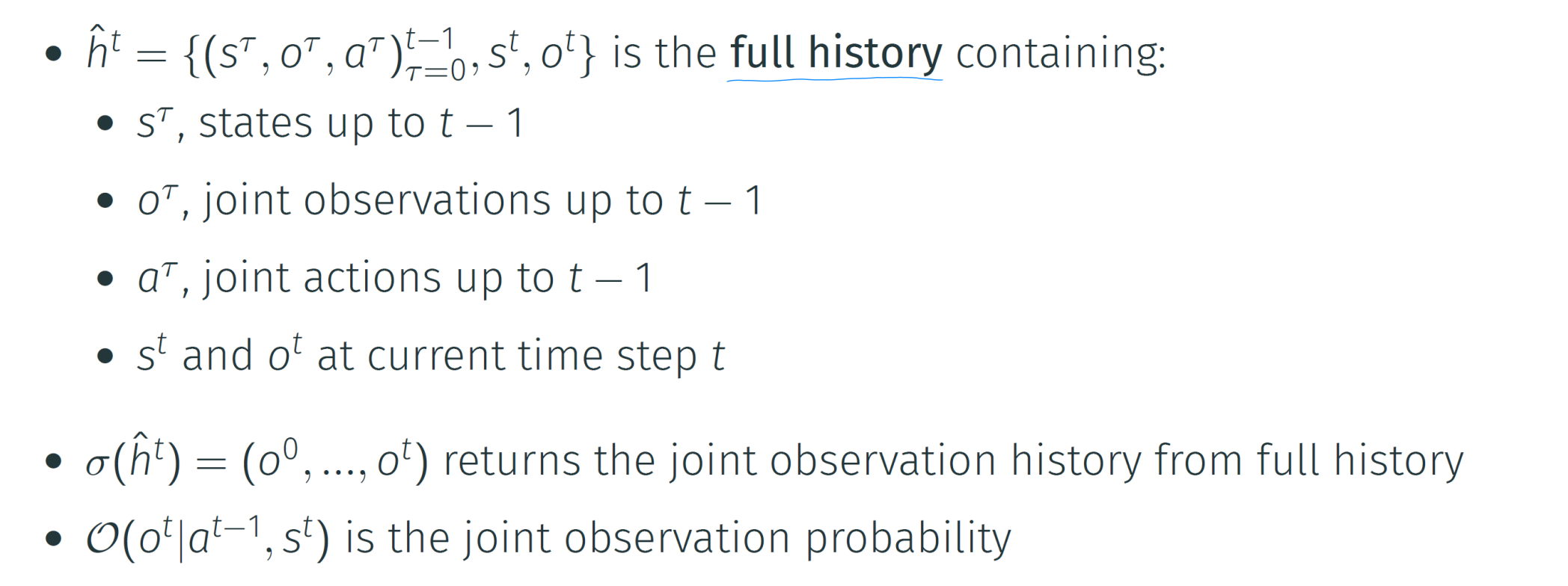
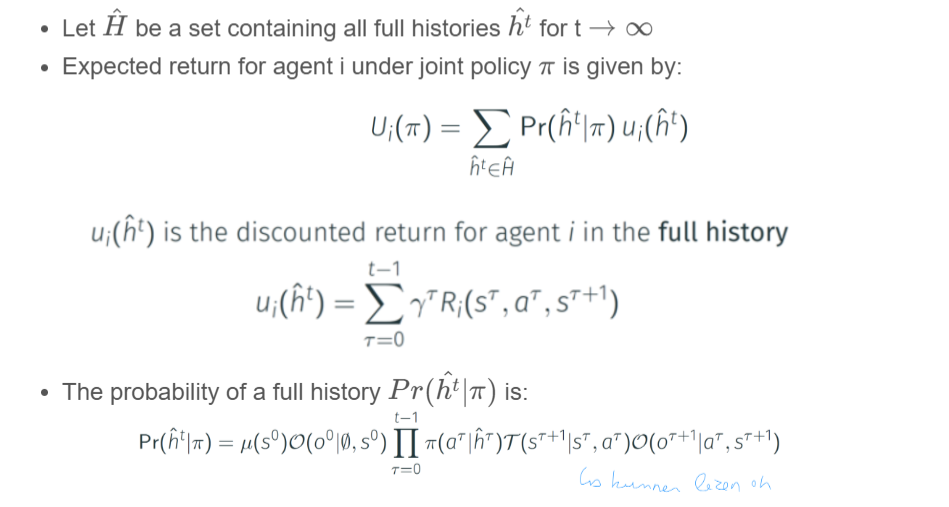
History-based expected return

In een POSG hebben agenten te maken met partiële observaties. Ze zien de volledige toestand van de wereld (s) niet direct. Om toch goed te kunnen voorspellen wat de gevolgen van acties zijn, moet een agent kijken naar de volledige geschiedenis (h^t) van wat er tot nu toe is gebeurd, in plaats van alleen het huidige moment.

Given a joint policy π, we can define the expected return for agent i under ππ as the probability-weighted sum of returns for agent i under all possible full histories.

Dit betekent:

• ui​(h^t): De daadwerkelijke, verdisconteerde beloning (discounted return) die agent i ontvangt in één specifieke geschiedenis/traject.

• Pr(h^t∣π): De waarschijnlijkheid dat deze specifieke geschiedenis zich voordoet als iedereen policy π volgt. Deze kans hangt af van de transitiefunctie van de omgeving en de policies van alle agenten.

Recursive formulation of expected return

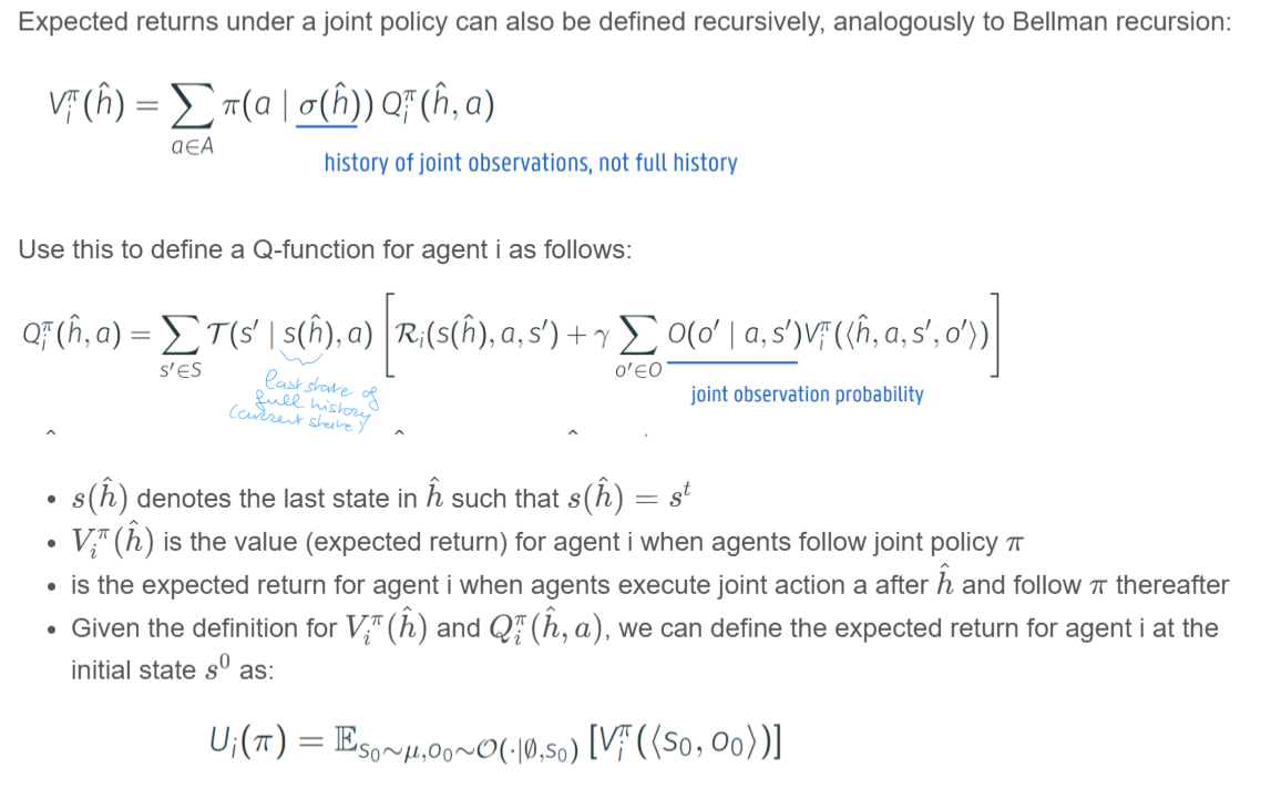
Net als in single-agent RL, kan deze opbrengst recursief worden berekend (analoog aan de Bellman-vergelijking), maar dan geconditioneerd op de geschiedenis in plaats van alleen de staat:

• Viπ​(h^): De waarde van agent i gegeven een geschiedenis h^.

• Qiπ​(h^,a): De verwachte opbrengst als na geschiedenis h^ de gezamenlijke actie a wordt uitgevoerd.

Samenvattend verschuift de focus in MARL van "wat is de waarde van deze toestand?" naar "wat is de waarde van deze geschiedenis?", omdat de geschiedenis de enige betrouwbare basis is voor besluitvorming in een gedeeltelijk waarneembare wereld.

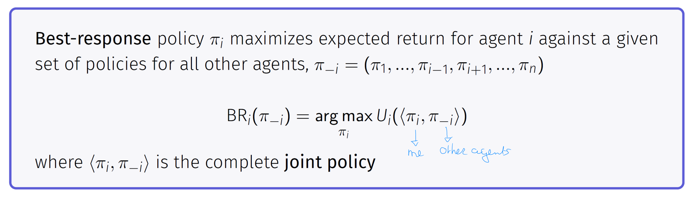
Best response

Many solution concepts are expressed compactly based on best responses

Equilibrium solution concepts

• minimax

Minimax is a solution concept defined for two-agent zero-sum games. Recall that one agent's reward is the negative of the other agent's reward.

• The existence of minimax solution in normal-form games was first proven by John von Neumann (1928)

• Minimax solutions also exist in two-agent zero-sum stochastic games with finite episode lengths, like chess and Go

Definition:

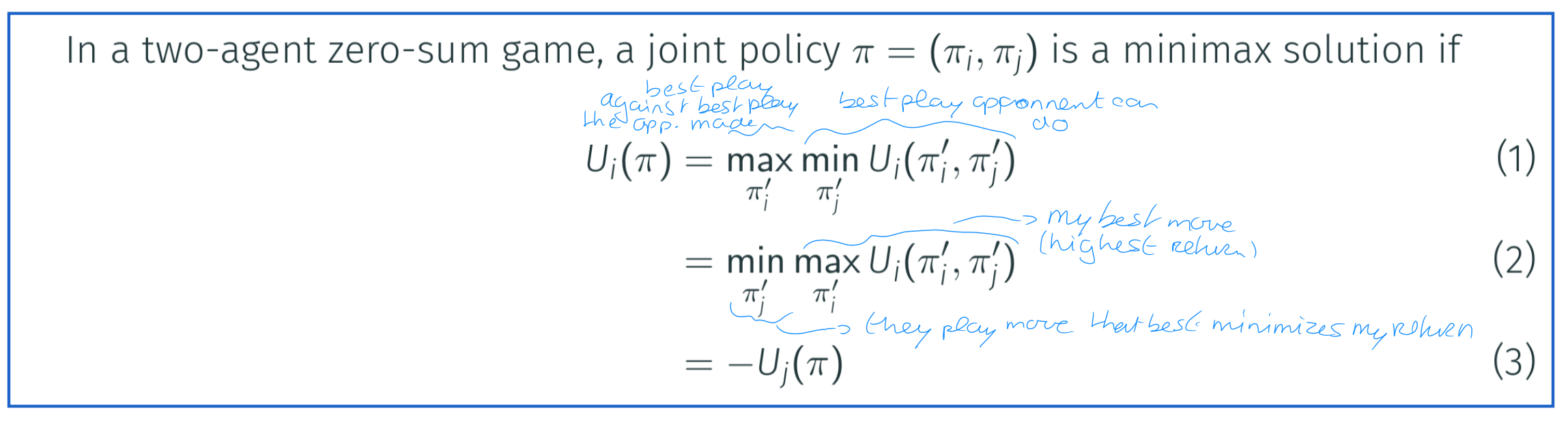
• Eq.1 is the minimum expected return agent i can guarantee against any opponent

• Eq.2 is the minimum expected return agent j can force on agent i

• A minimax solution is the best response to the worst-case opponent

• (πi,πj) is a minimax solution if πi∈BRi(πj) and πj∈BRj(πi)

Equilibrium solution concepts

• nash equilibrium

Nash equilibrium solution concept applies the idea of a mutual best respones to general-sum games with two or more agents.

• No agent i can improve its expected returns by changing its policy πiπi​ assuming other agents policies remain fixed:

  

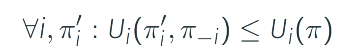
• Each agent's policy is a best response to all other agent's policies

• John Nash (1950) proved the existence of such a solution for general-sum non-repeated normal-form games

An agent following Nash strategy is guaranteed to do no worse than a tie (in expectation).
Plays perfect defense, and wins when the opponent makes a mistake.

Shortcomings of Equilibruim solutions

Equilibrium solutions are standard solution concepts in MARL, but have limitations.

• Sub-optimality:

  • nash equilibria do not always maximize expected returns

  • E.g. in prisoners dilemma, (D,D) is Nash but (C,C) yields higher returns

• Non-uniqueness:

  • there can be multiple (even infinitely many) equilibria, each with different expected returns

• Incompleteness

  • Equilibria for sequential games don't specify actions for off-equilibrium paths, i.e. paths not specified by equilibrium policy Pr(ht^∣π)=0

  • If there is a temporary disturbance that leads to an off-equilibrium path, the equilibrium policy ππ does not specify actions to return to a on-equilibrium path.

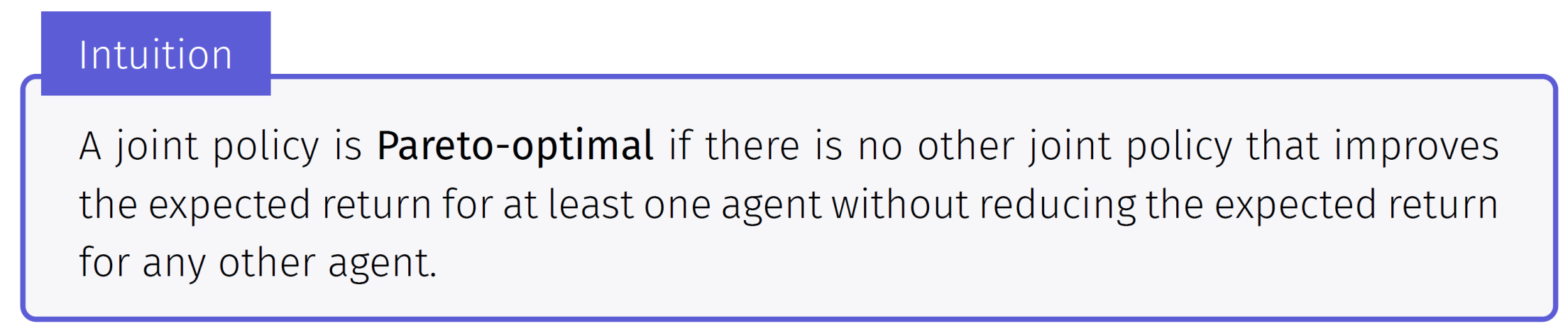
Pareto optimality

To address some of these limitations, we can add additional solution requirements such as Pareto optimality.
A joint policy π is Pareto-optimal if it is not Pareto-dominated by any other joint policy. A joint policy π is Pareto-dominated by another policy π′ if

Welfare optimality

Dit concept richt zich op het maximaliseren van het totale nut voor de groep.

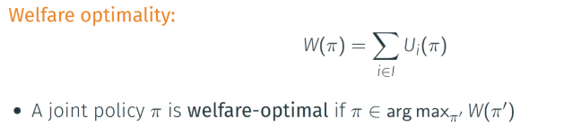
• concept only useful in general-sum games

• Een gezamenlijke strategie (policy π) is welvaartsoptimaal als de som van de verwachte opbrengsten (Ui​) van alle agenten maximaal is:

• Deze oplossing is per definitie Pareto-optimaal, maar houdt geen rekening met de verdeling; het is mogelijk dat één agent alles krijgt en de rest niets, zolang het totaal maar het hoogst is,.

Fairness optimality

Dit concept richt zich op een evenwichtigere verdeling van de beloningen.

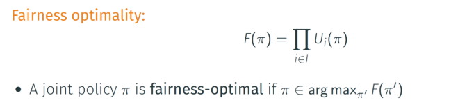
• concept only useful in general-sum games

• Een gezamenlijke strategie is eerlijkheidsoptimaal als het product van de verwachte opbrengsten van alle agenten maximaal is:

• Door te vermenigvuldigen wordt vermeden dat agenten een beloning van 0 krijgen (omdat het totale product dan 0 zou zijn). Dit dwingt het systeem om oplossingen te zoeken waarbij elke agent profiteert,.

Relations between solution criteria

1. Welfare optimality implies Pareto optimality

(Welvaartsoptimaliteit impliceert Pareto-optimaliteit)

• De logica: Welvaartsoptimaliteit betekent het maximaliseren van de totale som van de beloningen van alle agenten (W(π)=∑Ui​).

• De relatie: Als je een oplossing hebt die de totale som maximaliseert, is het per definitie onmogelijk om de beloning van één agent te verhogen zonder die van een ander te verlagen (anders zou de som immers nog hoger kunnen worden). Daarom is een welvaartsoptimale oplossing automatisch ook Pareto-optimaal.

2. Pareto optimality does not imply welfare optimality

(Pareto-optimaliteit impliceert geen welvaartsoptimaliteit)

• De logica: Pareto-optimaliteit betekent slechts dat je de situatie van niemand kunt verbeteren zonder iemand anders te schaden. Dit zegt niets over de totale som.

• De relatie: De "Pareto frontier" (de verzameling van alle Pareto-optimale punten) bevat vele mogelijke verdelingen. Een punt op deze lijn kan een lage totale som hebben (bijvoorbeeld een verdeling die heel gunstig is voor één agent maar slecht voor de rest), terwijl een ander punt op diezelfde lijn een veel hogere totale som heeft. Niet elk Pareto-punt is dus het punt met de hoogste totale welvaart.

3. Fairness optimality does not imply Pareto optimality

(Eerlijkheidsoptimaliteit impliceert geen Pareto-optimaliteit)

• De definitie: In de slides wordt eerlijkheid gedefinieerd als het maximaliseren van het product van de beloningen (F(π)=∏Ui​).

• De relatie: Hoewel dit vaak leidt tot Pareto-optimale oplossingen in scenario's met positieve beloningen (omdat een hoger product vaak samenvalt met efficiëntie), geldt dit niet altijd in algemene zin (bijvoorbeeld bij negatieve beloningen of specifieke spelstructuren). De bronnen stellen expliciet dat eerlijkheidsoptimaliteit Pareto-optimaliteit niet garandeert.

    ◦ Context: Als beloningen negatief zijn (zoals strafjaren in het Prisoner's Dilemma), kan het maximaliseren van het product leiden tot een keuze voor twee grote negatieve getallen (bijv. −5×−5=25) boven twee kleine negatieve getallen (bijv. −2×−2=4), wat duidelijk niet Pareto-optimaal is (want -2 is beter dan -5).

4. Pareto optimality does not imply fairness optimality

(Pareto-optimaliteit impliceert geen eerlijkheidsoptimaliteit)

• De logica: Een Pareto-optimale oplossing kan extreem oneerlijk zijn.

• De relatie: Een situatie waarin één agent alles krijgt en de andere agenten niets (bijvoorbeeld beloningen 100 en 0), is vaak Pareto-optimaal (je kunt de agent met 0 niets geven zonder van de agent met 100 af te nemen). Echter, de "fairness score" (het product) zou hier 0 zijn. Pareto-optimaliteit garandeert dus geen eerlijke verdeling of een maximaal product.

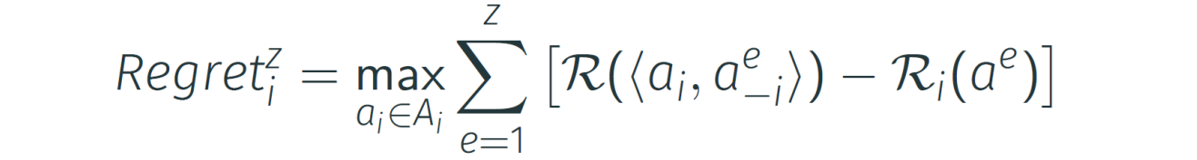
What is regret

Regret is een metriek die achteraf (in hindsight) meet hoe goed een agent heeft gepresteerd ten opzichte van de best mogelijke strategie die hij had kunnen kiezen, gegeven de acties van de tegenstanders.

• Definitie: Het is het verschil tussen de beloning die de agent daadwerkelijk heeft ontvangen en de beloning die de agent zou hebben ontvangen als hij de beste actie (of policy) had gekozen tegenover de vaste keuzes van de andere agenten in het verleden,,.

• Intuïtie: Stel dat je een reeks spelletjes Steen-Papier-Schaar hebt gespeeld. Achteraf kijk je terug en bereken je: "Hoeveel vaker had ik gewonnen als ik altijd Steen had gespeeld tegen jouw acties? Of altijd Papier?" De strategie die het meeste had opgeleverd wordt vergeleken met wat je werkelijk deed. Het verschil in score is je 'regret'.

• Formule: Voor een reeks episodes z wordt de totale regret gedefinieerd als het maximum van de cumulatieve verschillen tussen de optimale beloning (met kennis achteraf) en de ontvangen beloning,.

What is no regret

No-Regret is een eigenschap van een leer-algoritme. Een algoritme wordt gezien als een "no-regret" algoritme als het garandeert dat de agent op de lange termijn leert van zijn fouten.

• De voorwaarde: Er is sprake van no-regret als de gemiddelde regret per episode naar nul (of lager) gaat naarmate het aantal episodes (Z) naar oneindig gaat (Z→∞),.

• Betekenis: Dit betekent niet dat de agent nooit verliest of fouten maakt. Het betekent dat de agent uiteindelijk minstens zo goed presteert als de beste statische strategie die hij had kunnen kiezen tegen de geschiedenis van de tegenstander. De agent blijft niet structureel fouten maken die hij had kunnen vermijden.