Multiple Linear Regression

Limitations of MLR

1. conclusion & inferences made only valid for the data range used

2. Cant make causation statements (X causes Y)

3. High R² doesn’t guarantee it will be good fit for other data

R²

measures fit of regression line into the data

• higher value shows large portion of variability in dependent variable

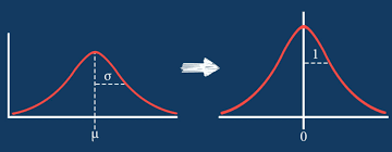
Standardized data

data than can be transformed to have a mean of 0 and a SD of 1 for each variable

Slope

shows increase change of y for one unit increase in x

Regression vs. residual

regression is a method used to find line of best fit (it is the line of best fit

residual is the distance of data pt from regression line

Coefficient table variables

1. Unstandardized Coefficient (B): shows that increase of 1 unit of the independent variable is equal to the B increase of dependent variable

2. Standardized Coefficient (β): shows 1 SD increase of indep. variable is equal to B SD increase of dep. variable

   • higher β = stronger effect

   • 0.7 - 1+ β value is strong effect

3. Significant (p < ): shows statistical significant at lvl

R

represents correlation coefficient

• shows strength & direction of linear relationship btenwee 2 variables

Durbin Watson

detects autocorrelation in the residuals of the linear regression model

• examines if a residual is correlated with the previous residual

• goes from 0-4, with 2 showing zero correlation

• close to 2 - no correlation

• 2+ = positive autocorrelation (residuals similar over time)

• 2- = negative autocorrelation (residuals switch signs)

Pearson correlation

Tells strength and direction of linear relationship between 2 variables (-1, 0, 1+)

Simple linear regression equation to solve for mean

Y^= b0​ + b1​ * X

x = independent variable (waist circumference)

b0 and b 1= dependent variable points (fasting glucose)

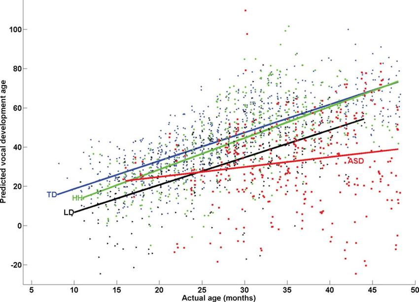
Between Group Differences

Looking at differences between stuff

• ex: one species of penguin heavier than others

• other specie penguin have longer flippers

• visual differences affects results (cant treat all penguins the same)

If differences are only in intercepts (start same with effect staying same across groups) the species is included as a main effect

If differences are also in slopes (effect changes depending on species) interaction term is added for moderaton

Within Group Differences

When relationship not same for each species, one line can’t be used for the species

• different line for each species with intercept & own slope

“species moderate the relationship”: species changes the affect of variable

• within group differences are the fuel as even with one type, the species is different

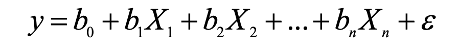
Multiple Linear Regression

Model to predict the value of 1 variable from another

• used to predict values of an outcome from several predictors

Equation of the variation of a straight line

y = b0 +b1 * x

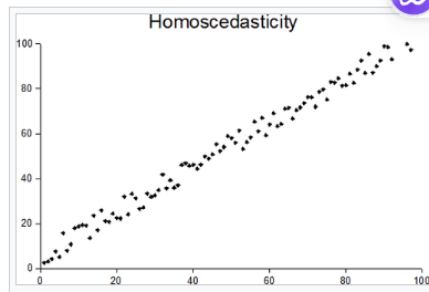
MLR Assumptions

1. Linear relationship between dependent & independent variables

2. Homoscedasticity is assumed (spread of the data stays same at every lvl of independent variable)

   • data pts follow trend with same variance

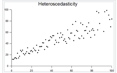
Heteroscedasticity

Data pts in mlr shows variance of y value of dots increase as x values increase

• data points start getting more spread out but with same pattern

Collinearity

In a mlr where 2 or more predictors (independent) variables are highly linear related

• 1 variable can be almost perfectly predicted from another variable

Predictors in MLR

they are the independent variables (can be multiple like age, sex, etc.)

Multicollinearity

When predictors aren’t exactly, but highly, linearly related

Variance inflation factor (VIF)

Shows how much variance is inflated due to multicollinearity

• VIF = 1 = no correlation with other vairables

• VIF = 1 - 5 = moderate correlation

• VIF > 5-10 = potential multicollinearity issues