Applied econometrics 2 lectures 5-6 - Forecasting

Caveat of forecasting

Possible structural breaks in economic conditions are not accounted for by our forecasting models

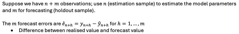
In-sample period / estimation period

The sample period over which the models are estimated.

Out-of-sample period / hold-out sample

the data segment we hold out in order to evaluate the estimated models for predictive power

Forecast origin

The exact time period at which the forecast is being made - y_n

WE USE n INSTEAD OF t y_n NOT y_t

Forecast horizon

The amount of time between the forecast origin and the event being predicted

one-step-ahead forecasts

When the forecast horizon is one period → y^{^}_n+1

Point forecasts

These estimate a particular value of the variable being forecast

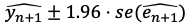
Forecast intervals

intervals within which the forecasted value should be found for a particular percentage of the time

e.g. similar to 95% confidence intervals

point forecast +/- Critical value * SE

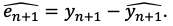
Forecast error

the difference between actual (observed) value of the variable and its predicted value.

Forecasting steps

1. Estimate several ARDL (p,q) models by varying p and q based on the in-sample period

2. For all models, check for serial correlation, and eliminate the models with serial correlation

a. Use Breusch-Godfrey test

3. For all surviving models, keep the one which best fits the in-sample data

a. Use model selection criteria (AIC or BIC) → smallest is best

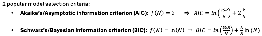
Model selection criteria

We want to maximize how well the model fits the data (minimize squared residuals) but penalize a greater number of regressors

IC = ln (SSR / n) + k/n * f(n)

f(n) - determines the penalty from adding more regressors otherwise you could have as many regressors as data points

95% Forecast interval

Where errors come from in forecasting

Variation from sampling → arises from coefficients being estimated

Roughly proportional to T^-1/2 T - time periods used

Variation from variance in the population (uncertainty in u_t)

•     Does not change with sample size → generally it is the dominant term of SE

Standard error of forecast error

How to evaluate model based on forecast performance

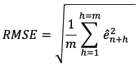
- root mean squared error (RMSE)

- mean absolute error (MAE)

Forecast errors for every forecast

root mean squared error (RMSE)

– Essentially the sample standard deviation of the forecast error

– Choose model with smallest RMSE → Smaller is better

mean absolute error (MAE)

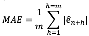
– Average of the absolute forecast error

– Smaller is better again

Lag operator

Lags the variable by 1 period

L such that LX_t = LX_t-1

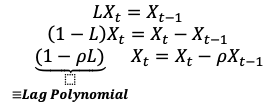
Lag polynomial

(1-pL)

For stability, the root of the lag polynomial must have an absolute value greater than one

Root of lag polynomial - L = 1 / p → require |p| < 1

What happens when |p| < 1

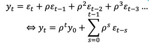
As t&s increase the effect of p decreases → when t→infinity, term = 0 so E(y_t) = 0 Constant

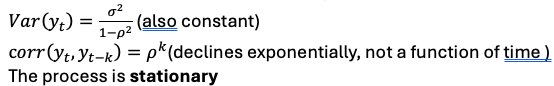
The impact of shocks (ε_t) fade over time

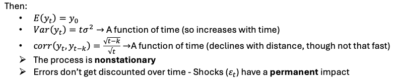
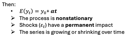
what happens when p = 1

Our model becomes a random walk

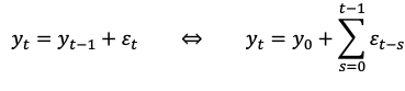
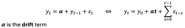
Random walk with drift

the random movement is around a linear trend

How to differentiate between AR(1) processes and processes with very high correlation

Let time pass → One reverts to mean of 0 and one doesn’t

Order of integration - I(0) vs I(1)

A weakly dependent process is “integrated of order zero,” or I(0)

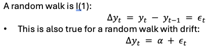
If the first difference of a non-stationary series is stationary. In this case, the series is “integrated of order one,” or I(1)

What if the series is integrated of order 1 - I(1)

– Standard inference doesn’t work

– Can be used in regression analysis after first-differencing

Both random walk & random walk with drift are I(1)

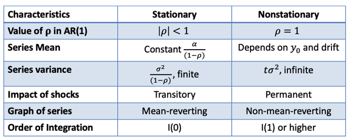
Stationary & nonstationary series overview

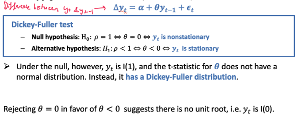
Dickey-Fuller test

Tests for a unit root

1 sided test (p<1)

Rejecting null = NO unit root

DF critical regions are different to t tests

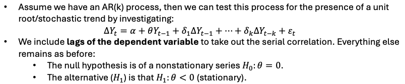
Augmented DF test

Our Dickey-Fuller (DF) test may mistake serial correlation for unit root behaviour so ADF washes out autocorrelation

Issues with time series unit root tests

The time-series test might not reject H_0 but we still doubt the data is I(1):

• Low power of the test in near-unit root case

  • An AR1 process with a very high correlation coefficient and a unit root process, their realisations might look very similar if you don't have enough time periods

• Inference is sensitive to treatment of serially correlated errors and treatment of means and trends

• Sensitivity to structural breaks

• Non-linearities

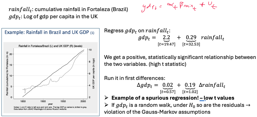
Spurious regression

Situation in which x and y are not related in any way, but an OLS regression using the usual t statistics will often indicate a relationship

How Non-stationary time series create spurious regressions

• If we omit a time trend - A special case of Omitted Variable Bias

• If we are regressing I(1) series, even if they are independent

  • As T increases, we reject a true null more often than we should

Example of spurious regression