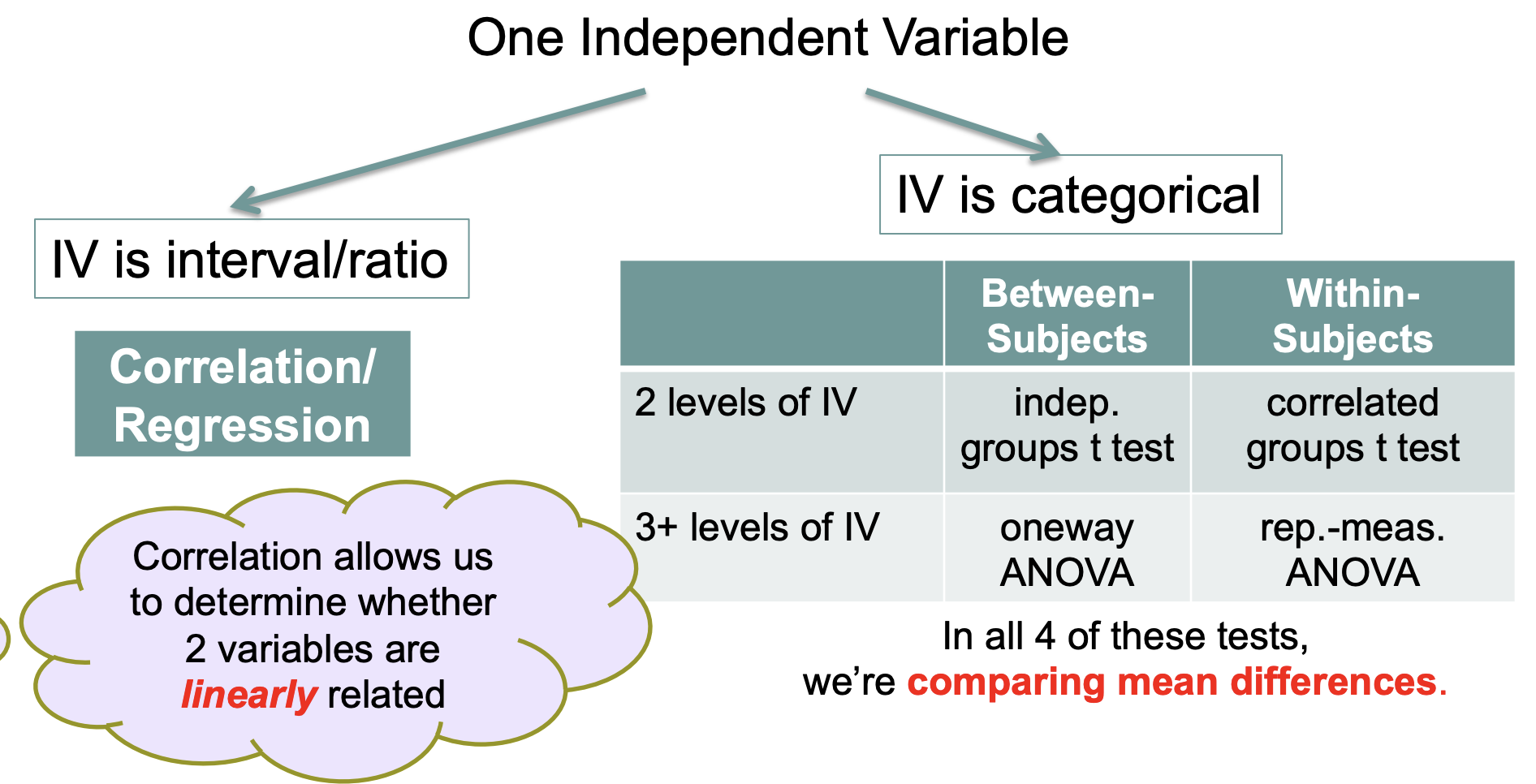
Correlation/ Regression

Putting Correlation / Regression into Context

DV = interval/ratio

Three Characteristics of a Correlation (r) Between X & Y

Direction: positive, negative, no correlation

Degree / magnitude: ranges from -1 to +1; extreme scores unlikely

• Possible ranges of r values [-1 to +1] perfect negative correlation to perfect positive correlation… correlations closer to -1 or +1 = points are closer to the regression line… unlikely to get a correlation of ±1 because… measurement error, Y is predicted by more than just 1 X variable

Form: correlation useful only for linear relationships

Important note

Before conducting statistical analyses (e.g., calculating r), always look at your x and y data by producing a scatterplot!

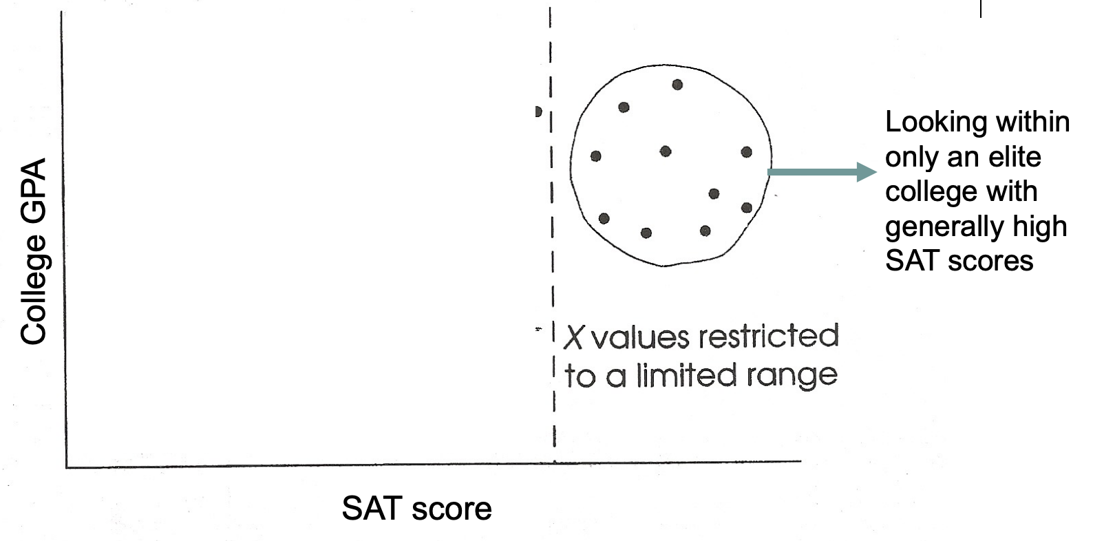
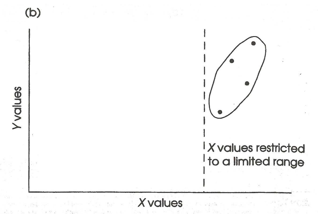
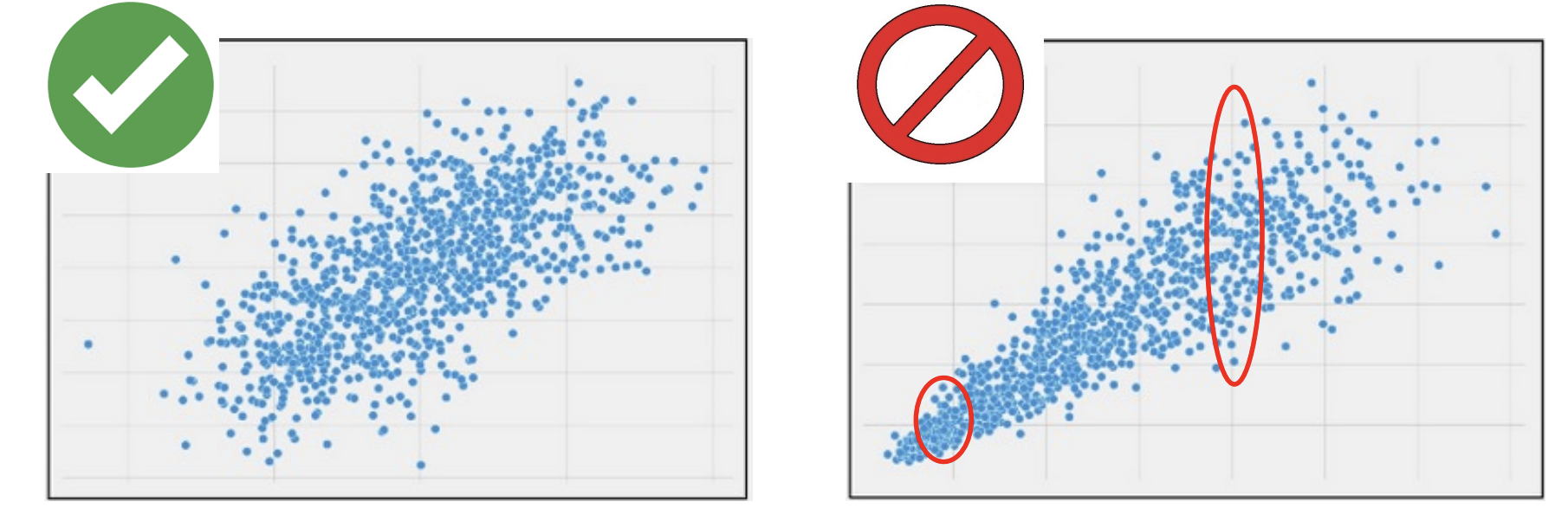
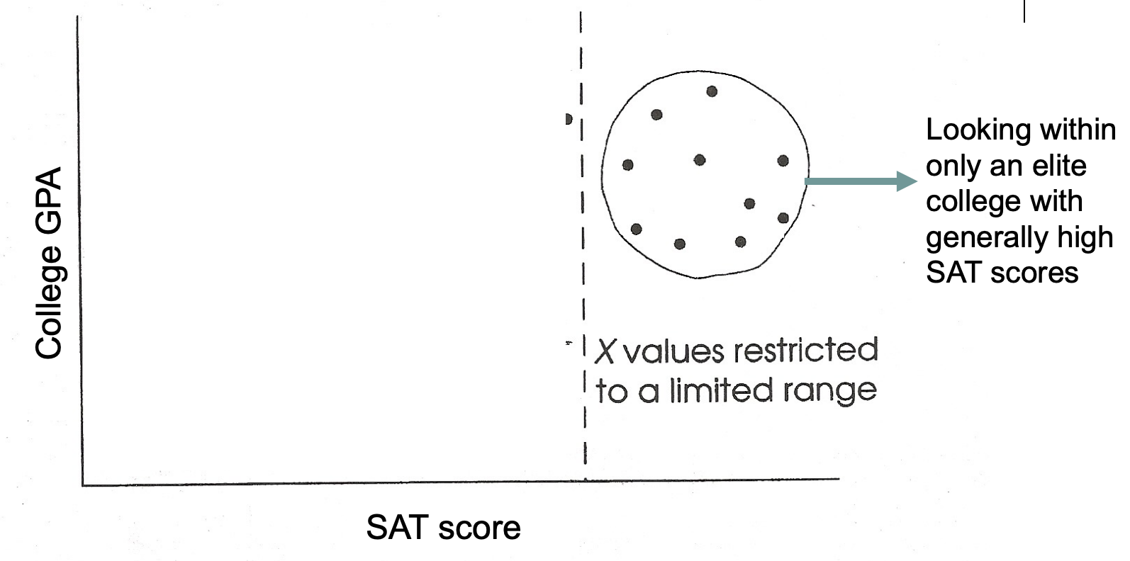
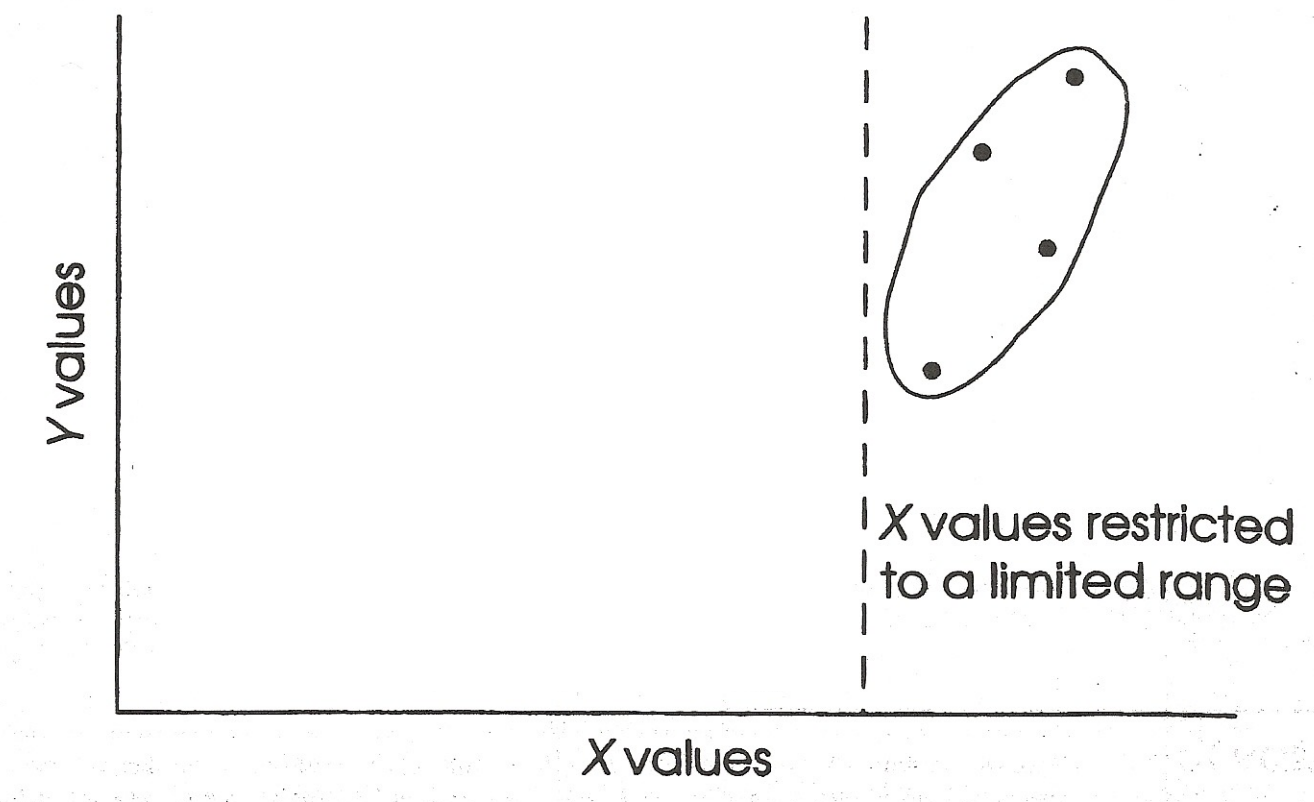
Problems to Watch Out For: Restricted Range

• Occurs when experimenters look at only one portion of the data (not good)

• Can lead to underestimation of a relationship between X and Y

• Can lead to overestimation of a relationship between X and Y

Restricted Range: Case 1

• Underestimation of association

  • Strong linear relationship when full range of x values is used, but no relationship when restricted range used

Restricted Range: Case 2

• Underestimation of association

  • Strong linear relationship when full range of x values is used, but no relationship when restricted range used

Restricted Range: Case 3

• Overestimation of association

  • No relationship when full range of x values is used, but strong relationship when restricted range used

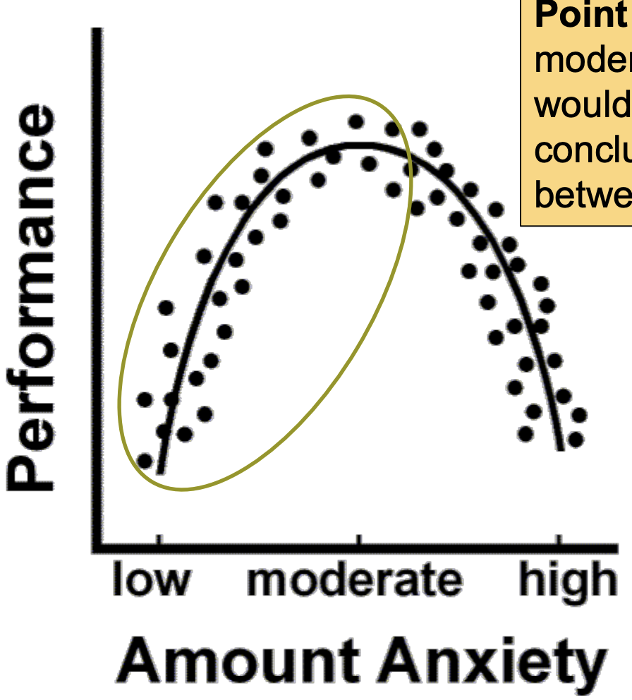
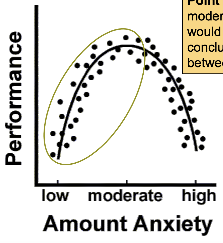
Non-linear relationships: Example 1

Curvilinear relationship:

• If we looked only at low to moderate levels of anxiety, we would come to an erroneous conclusion about the relationship between anxiety and performance.

• To be safe, use a wide range of X and Y values, and do not make conclusions based on extrapolation beyond your observed values of X

• SIDE NOTE: I will ask you to extrapolate when you calculate the regression line, though.

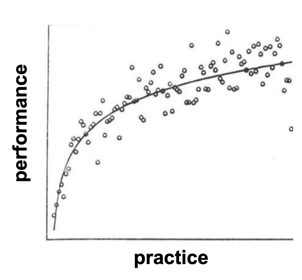
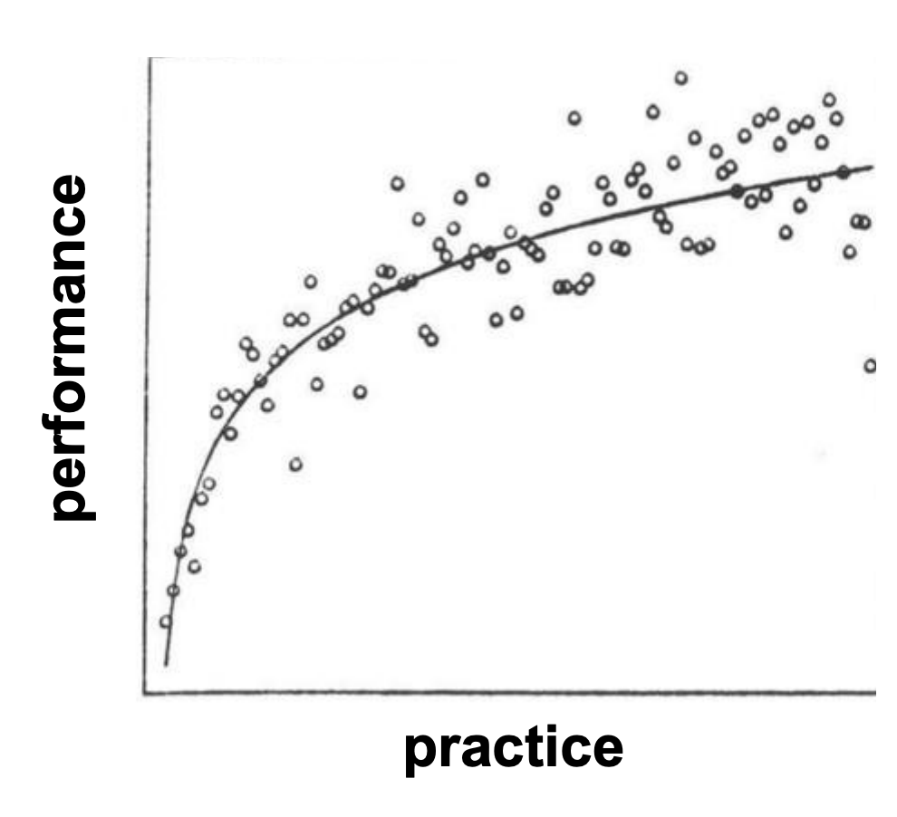
Non-linear relationships: Example 2

• These data are not linear (the curve levels off – is asymptotic)

• Here, the change in the y-values become increasingly small as the x-values increase.

Problems to watch out for: Outliers

• Scores that are outside the range for X, Y, or both

• Can cause either over or underestimation of the correlation

Outliers: Overestimation of association

Including the outlier (inaccurately) strengthens the correlation.

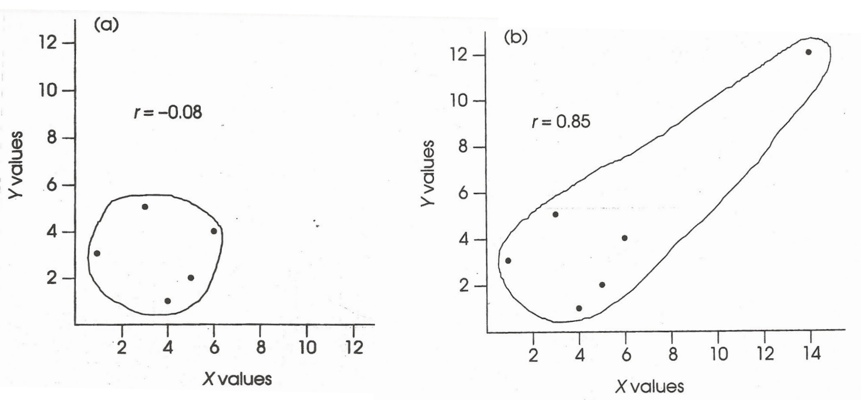
Outliers: Underestimation of association

In this case, including the outlier weakens the correlation

Bottom line: set criteria for outlier removal BEFORE plotting/ analyzing the data; do not tempt yourself into selective data trimming!

The Pearson Product-Moment Correlation (r) - Conceptual Understanding

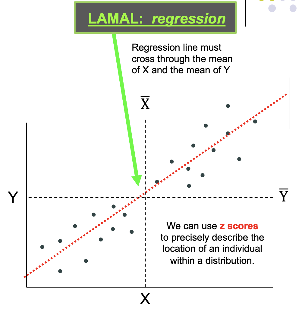
r is an indicator of location in X distribution (relative to mean of X)

& location in Y distribution (relative to mean of Y)

Regression line must cross through the mean of & the mean of Y

We can use z scores to precisely describe the location of an individual within a distribution.

• For a positive correlation: positive Z scores on X correspond to positive Z scores on Y; negative Z scores on X correspond to negative Z scores on Y.

• For a negative correlation, positive Z scores on X correspond to negative Z scores on Y and vice-versa.

• We cannot just use ∑ZXZY as a measure of r because of the same drawback we ran into with the SS…

• It keeps getting larger and larger as the number of scores increases. But.. Use same solution (divide by N-1)

Definitional formula for r

SSxy = SP = Sum of Products: How much X and Y covary

Remember: SS = how much a set of scores varies from its mean.

So we will use… SSX for variable X SSY for variable Y.

r assesses how the covariation of X and Y relates to the variation (variability) of X and Y separately

Unlike sum of squares, covariance CAN be negative! (i.e., as X increases, Y decreases).

When the covariation (numerator) is big, r is big.

Understanding r / r vs. slope

Value of r = .72→ A 1 unit increase in X is associated with, on average, a .72 unit increase in Y.

r and the slope of a line (b) are similar, but not the same.

r is in standard deviation units, whereas the slope of a line (b) is the rise over run (e.g., the change in X over the change in Y), and is in scale units.

Inferential Aspects of Correlation (i.e., “Is r significant?”)

BUT… we can get a big r in our sample even when there’s no relationship between X and Y in the population… BECAUSE… a large r could occur as a result of sampling error alone. So we need to check whether or not our r is statistically significant.

Statistics vs. Parameters

For a sample: correlation = r

For a population: correlation = ρ (rho)

Steps in Hypothesis Testing; Null & Alternative Hypotheses

H0: ρ = 0 (there is NO linear relationship in the population) H1: ρ ≠ 0 (there IS a linear relationship in the population)

Steps in Hypothesis Testing: Constructing a Sampling Distribution

Pull all possible random samples of size N (where a sample is a set of X,Y scores) from a single population, calculate the r values, and plot the r values in a histogram.

What are df?

What are df for a correlation?

We lose a df for each mean we estimate (i.e., one for X and one for Y)

So, df = N – 2

Our 3 Qs:

Is there a relationship?

• Is the correlation significant? (no leading 0s!)

If so, what is the nature of that relationship?

• Is the correlation positive or negative?

• Describe in words using the context of the example, i.e. Disgust and conservatism were positively correlated; in other words, stronger feelings of disgust were associated with greater political conservatism

If so, what is the strength of that relationship?

Strength of the Relationship between X & Y

We can’t just use the magnitude of the correlation coefficient (r) as a measure of strength.

• the same r can be big in one context and small in another, depending on N

• r isn’t linear (.8 isn’t twice as big as .4)

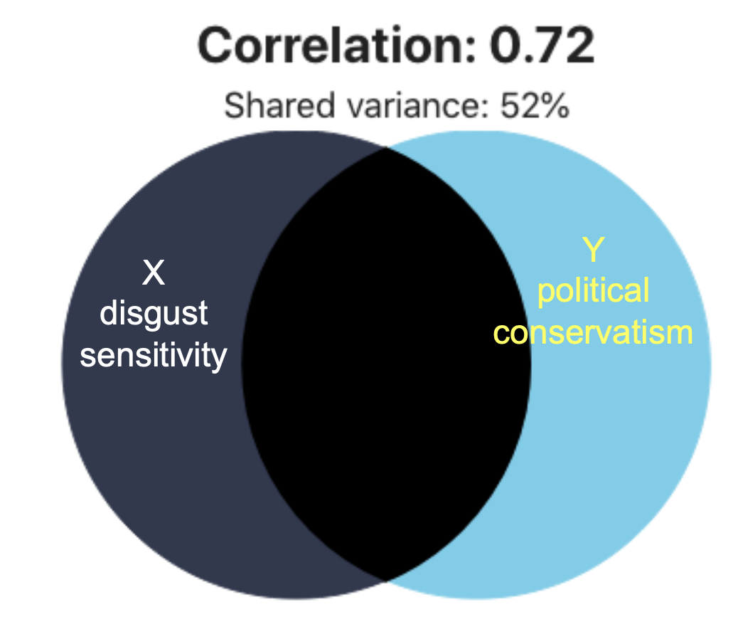
• Strength = Coefficient of determination = r²

• For our example, r² = (.721)² = .52

Because it is expressed as a proportion of variability, r² can be compared across studies

Coefficient of alienation

1 - r²; 1 - .52 = .48

proportion of variability in Y NOT explained by X; i.e., error

Assumptions of the Pearson Correlation

• Sample is independently and randomly selected from the population

• Bivariate normality:

  • The distribution of Y scores at any value of X is normal in the population

  • Robust to violations of this assumption if N > 15

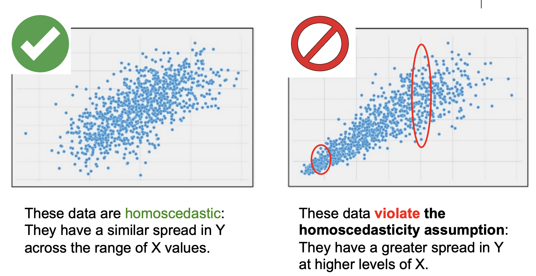
• Homoscedasticity:

  • Y scores have equal variances at each value of X in the population

  • Not robust to violations of this assumption

Data H→ They have a similar spread in Y across the range of X values.

No→ data violate the homoscedasticity assumption: They have a greater spread in Y at higher levels of X.

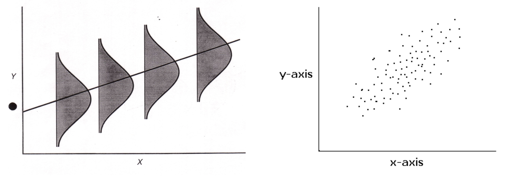
Bivariate Normality

Schematic of a bivariate normal dataset→ Picture this as a 3D graph, with the distributions coming out toward you.

An actual bivariate normal data set

Most of the scores fall close to the line of best fit.

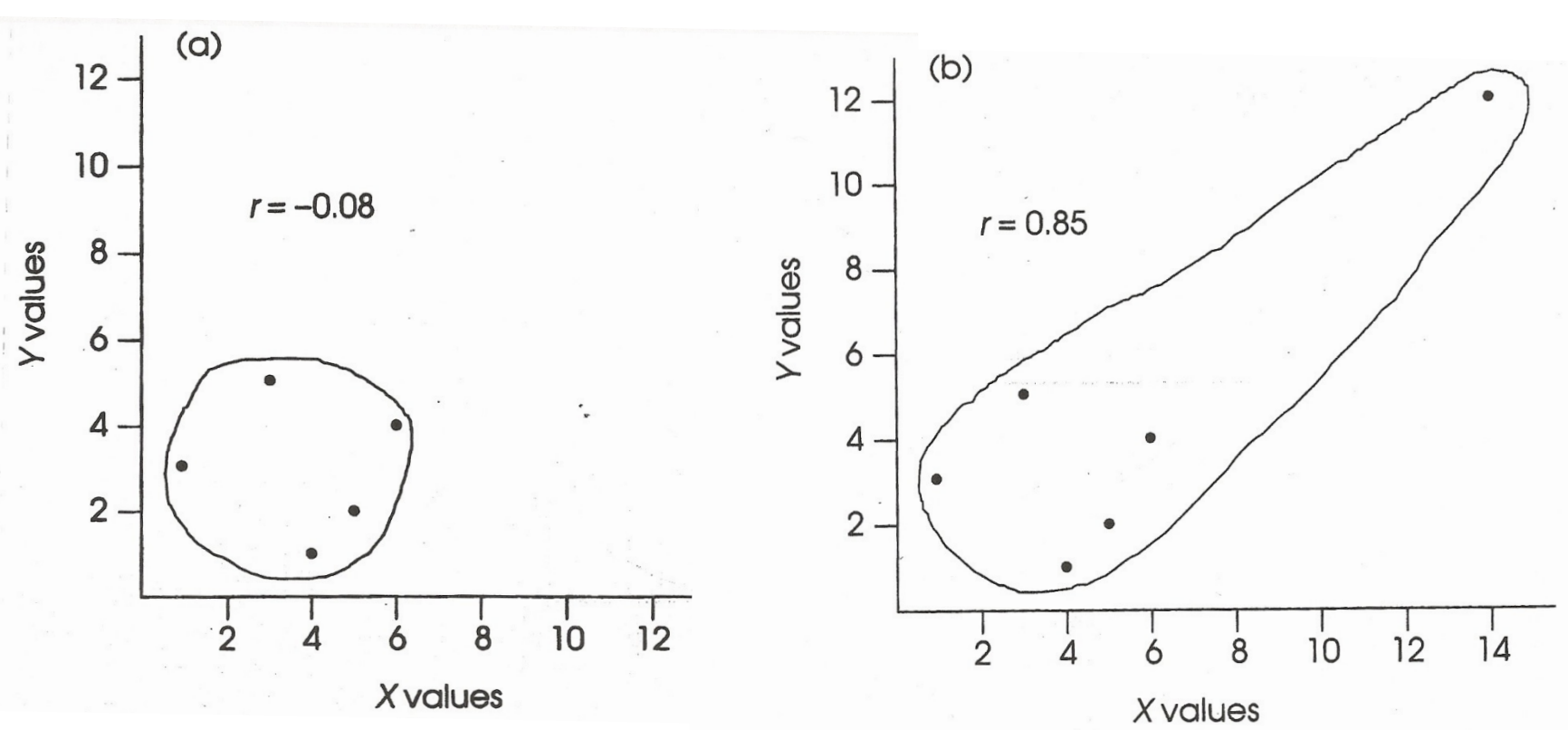
Visualizing Correlations

Notice that as r approaches 1, the data are closer and closer to the regression line.

Also consider: When r = -1 there is a perfect negative correlation between x and y

and: when r = 0 there is no correlation between x and y

…and here is what a scatterplot with a negative r looks like.

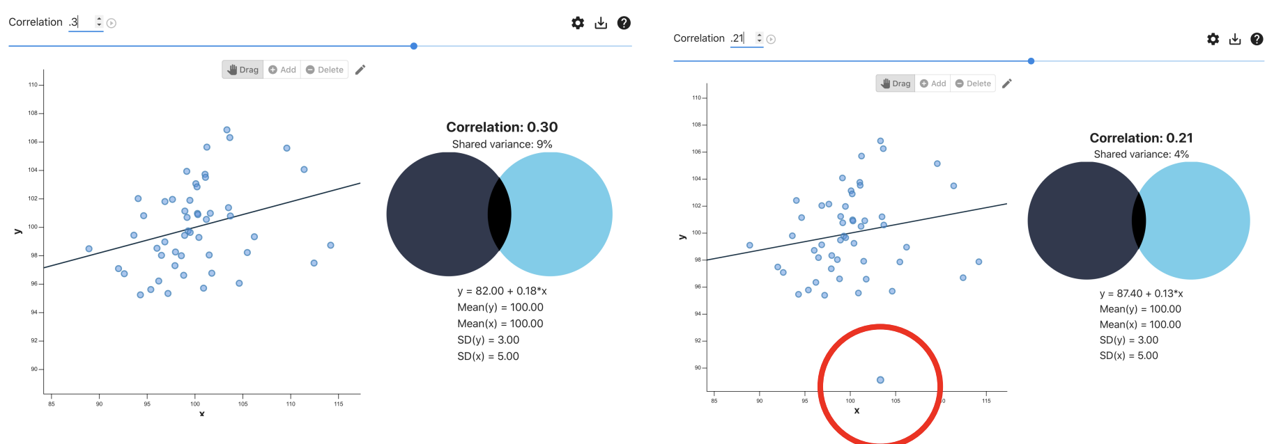
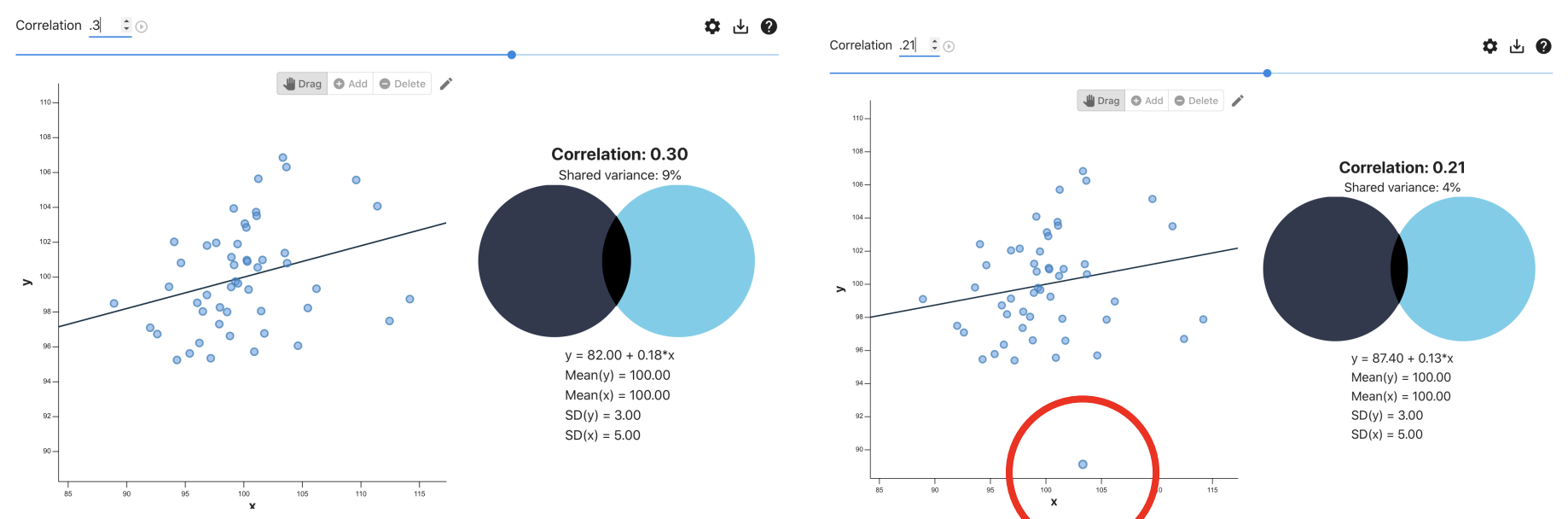
Interpreting r & r²

r = .3, r² = .09— We can explain about 9% of the variability in depression with loneliness

Problems to Watch Out For: Restricted range

• Occurs when experimenters look at only one portion of the data (not good)

• Can lead to underestimation of a relationship between X and Y

• Can lead to overestimation of a relationship between X and Y

Restricted range: Case 1: Underestimation of Association

Strong linear relationship when full range of x values is used, but no relationship when restricted range used

Restricted range: Case 2: Underestimation of Association

Strong linear relationship when full range of x values is used, but no relationship when restricted range used

Restricted range: Case 3: Overestimation of Association

No relationship when full range of x values is used, but strong relationship when restricted range used

Non-linear relationships: Example 1: curvilinear relationship

Point 1: If we looked only at low to moderate levels of anxiety, we would come to an erroneous conclusion about the relationship between anxiety and performance.

To be safe, use a wide range of X and Y values, and do not make conclusions based on extrapolation beyond your observed values of X.

SIDE NOTE: I will ask you to extrapolate when you calculate the regression line, though.

Point 2: These x and y data are not linear. Don’t conduct a correlation analysis on these data!

Non-linear relationships: Example 2

These data are not linear (the curve levels off – is asymptotic)

Here, the change in the y-values become increasingly small as the x-values increase.

Don’t conduct a correlation analysis on these data!

Problems to watch out for continued: Outliers

Scores that are outside the range for X, Y, or both

Can cause either over or underestimation of the correlation

Outliers: Overestimation of association

Including the outlier (inaccurately) strengthens the correlation.

Outliers: Underestimation of association

In this case, including the outlier weakens the correlation.

Bottom line:

• Always look at a scatterplot of your x and y data!

• Set your criteria for outlier removal BEFORE plotting or analyzing the data. Do not tempt yourself into selective data trimming!

The Pearson Product-Moment Correlation (r) - Conceptual Understanding

r is an indicator of location in X distribution (relative to mean of X)

and location in Y distribution (relative to mean of Y)

Regression: line must cross through the mean of X and the mean of Y

We can use z scores to precisely describe the location of an individual within a distribution.

So, for a positive correlation: positive Z scores on X correspond to positive Z scores on Y;

negative Z scores on X correspond to negative Z scores on Y.

For a negative correlation, positive Z scores on X correspond to negative Z scores on Y and vice-versa.

Statistics vs. Parameters

• For a sample: correlation = r

• For a population: correlation = p (rho)

What are the null & alternative hypotheses for a test of correlation?

H0: p = 0 (there is NO linear relationship in the population) H1: p ≠ 0 (there IS a linear relationship in the population)

Flashback: How did we construct the sampling distribution for the paired sample t test?

Pull all possible random samples of size N from a single population (where a sample is a set of difference scores), calculate the means, and plot the means in a histogram.

How do we construct the sampling distribution of r?

Pull all possible random samples of size N (where a sample is a set of X,Y scores) from a single population, calculate the r values, and plot the r values in a histogram.

3 Qs for every test:

• Is there a relationship? (i.e., is the correlation significant?)

• If so, what is the nature of that relationship?

  • Is the correlation positive or negative? (r = .72)

  • Describe in words using the context of the example:

  • Disgust and conservatism were positively correlated; in other words, stronger feelings of disgust were associated with greater political conservatism

  • If so, what is the strength of that relationship?

Strength of the Relationship Between X and Y

We can’t just use the magnitude of the correlation coefficient (r) as a measure of strength.

• the same r can be big in one context and small in another, depending on N

• r isn’t linear (.8 isn’t twice as big as .4)

• Strength = Coefficient of determination = r2

• For our example, r2 = (.721)² = .52 (no leading 0)

  • shared variance; 52% of the variability (SS) in political conservatism can be explained/predicted by disgust sensitivity (like h2!)

  • Because it is expressed as a proportion of variability, r² can be compared across studies.

Coefficient of alienation

1 - r²; proportion of variability in Y NOT explained by X; i.e., error

Assumptions of the Pearson Correlation

• Sample is independently and randomly selected from the population

• Bivariate normality:

  • The distribution of Y scores at any value of X is normal in the population

  • Robust to violations of this assumption if N > 15

Homoscedasticity

• Y scores have equal variances at each value of X in the population

• Not robust to violations of this assumption

Visualization of Homoscendasticity

1st— data are homoscendastic: they have a similar spread in Y across the range of X values

2nd— These data violate the homoscedasticity assumption: They have a greater spread in Y at higher levels of X.

What you need to conduct a regression analysis

1. You need the disgust scores (X = predictor variable)

2. X and Y need to be significantly correlated (r = sig).

3. You need the formula for the regression line

4. You need to do some simple math

THM: Regression allows you to be a bit more accurate than just relying on the mean of Y to predict the individual scores of Y.

Least-squares line

If you know someone’s disgust sensitivity score, and you have a least-squares regression line, you can predict any y value based on a given x value

Why is it called this?

Because it minimizes the squared vertical distances of the points to the line. — Should do a better job of predicting Y than just using the mean of Y

Regression involves finding the formula for the line that best predicts Y from X

Regression line vs. basic formula

Y = a + bX (where a = y intercept, b = slope)

vs

Ŷ = a+bX

The equation yields a predicted Y value for every X value rather than an actual Y value.

The line is a prediction, so the points don’t all fall exactly on the line; there will be error associated with the line.

b vs. r

b→ Describes the relation between X & Y in X & Y units

r→ Describes the relation between X & Y in standardized units (Z scores). An r of .72 means that a 1 SD change in X is associated with, on average, a .72 SD change in Y.

If you transform X & Y to Z scores before correlating them, r = b.

Formula for the y-intercept

We know that the regression line must go through the mean of the X ratings (IV; = 2.083) and the mean of Y ratings (DV; = 4.500)

So we can plug in the means for X and Y into our formula to calculate the Y intercept:

Plotting the least-squares line

Step 1. Select the lowest (0) & the highest (4) values of X.

Step 2. Plug in 0 for X to get the first Y value.

Step 3. Plug in 4 for X to get the second Y value.

Other than to calculate the Y intercept, do not extend your line past the values of X! Can’t extrapolate!

Accuracy of the Regression Line

What is the relationship between r and the accuracy of the regression equation?

• The bigger the r, the closer the points are to the line and the more accurate the regression equation

How do we evaluate how good our line is?

• Compute the standard error of estimate, which tells us, on average, how far the points fall (vertically) from the regression line