Intro To Quantitative Analysis - Decision Analysis

Multiple Choice Type Only

Quantitative Analysis

is a scientific approach to managerial decision making in which raw data are processed and manipulated to produce meaningful information

Raw Data → Quantitative Analysis → Meaningful Information

Quantitative Factors

are data that can be accurately calculated.

Examples:

• Different Investment Alternatives

• Interest Rates

• Invetory Levels

• Demand

• Labaor Cost

Qualitative Factors

are more difficult to quantify but affect the decision process.

Example:

• The weather

• State and federal legislation

• Technological Breakthroughs

The Quantitative Analysis Approach

(In Order)

1. Defining the Problem

2. Developing a Model

3. Acquiring Input Data

4. Developing a Solution

5. Testing the Solution (If failed, go back to step 2.)

6. Analyzing the Result (If failed, go back to step 2.)

Defining the Problem

Develop a clear and concise statement that gives direction and meaning to subsequent steps

• This may be the most important & difficult step

• It is essential to go beyond symptoms and identify true causes

• It may be necessary to concentrate on only a few of the problems — selecting the right problems is very important

• Specific and measurable objectives may have to be developed

Developing a Model

• Quantitative analysis models are realistic, solvable, and understandable mathematical representations of a situation

• Contain variables (controllable and uncontrollable) and parameters

• Scale Models

• Schematic Models

Different types of models:

Controllable Variables

are the decision variables and are generally unknown.

• How many items should be ordered for inventory

Parameters

are knwon quantities that are a part of the model

• What is the holding cost of the inventory?

Acquiring Input Data

Data may come from a variety of sources such as company reports, company documents, interviews, on-site direct measurement, or statistical sampling

Garbage In - Process - Garbage Out

Input data must be accurate — GIGO rule

Developing a Solution

The best (optimal) solution to a problem is found by manipulating the model variables until a solution is found that is practical and can be implemented

Common techniques are:

• Solving Equations

• Trial and Error — trying various approaches and picking the best result.

• Complete Enumeration — trying all possible values

• Using an algorithm — a series of repeating steps to reach a solution

Testing the Solution

Both input data and the model should be tested for accuracy before analysis and implementation

• New data can be collected to test the model

• Results should be logical, consistent, and represent the real situation

Analyzing the Results

Determine the implications of the solution:

• Implementing results often requires change in an organization.

• The impact of actions or changes needs to be studied and understood before implementation.

Sensitivity analysis

Determines how much the results will change if the model or

input data changes.

• Sensitive models should be very thoroughly tested.

Implementing the Results

Implementation incorporates the solution in the company

• Implementation can be very difficult

• People may be resistant to changes

• Many quantitative analysis efforts have failed because a good, workable solution was not properly implemented

Changes occur overtime, so even successful implementations must be monitored to determine if modifications are necessary.

Modeling in the Real World

Quantitative Analysis models are used extensively by real organizations to solve real problems

• In the real world, quantitative analysis models can be complex, expensive, and difficult to sell.

• Followign the steps in the process is an important compononent of success

Profit = Revenue - (Fixed Cost + Variable Cost)

Revenue — selling price per unit

Profit = sX - [f + vX]

The parameters of this model are f,v, and s. The decision variable is X.

Formula for profit.

Break-Even Point (BEP)

is the number of units sold that will result in $0 profit.

0 = sX - f - vX

1. They represent reality.

2. They help decision makers formulate problems

3. They provide meaningful information

4. They save time and money in decision making

5. They solve large / complex problems

6. They can be useful to multiple similar problems

What are the advantages of Mathematical Modeling

Deterministic Models

are mathematical models that do not involve risk.

• All of the values used in the model are known with complete uncertainty

Probabilistic Models

Mathematical modles that involve risk, chance, or uncertainty

• values used in the model are estimates based on probabilities

Defining the Problem

• problem not easily identified

• conflicting view points

• impact on other departments

• outdated solution

Developing a Model

• manager’s perception may not fit a textbook model

• trade-off between complexity and easy to understand

Acquiring Input Data

• data may not be collected for quantitative problems

• validity of data

Developing an Appropriate Solution

• math is hard to understand

• having only one answer may be limiting

Testing the Solution for Validity

Analyzing the Results in Terms of the Whole Organization

Possible Problems in Quantitative Analysis Approach

Probability

is a numerical statement about the likelihood that an event will occur.

1

The sum of the simple probabilities for all possible outcomes of an activity must equal —

Objective Probability and Subjective Probability

Types of Probability

Relative Frequency

Typically based on historical data (number of occurrences / total number of trials)

Classical or Logical Method

Logically determine the probabilities without trials (tails or head)

Subjective Probability

is based on the experience and judgment of the person making the estimate.

• Opinion polls

• Judgment of experts

• Delphi Method

Mutually Exclusive

Events are said to be —- if only one of the events can occur on any one trial

P (A | B) = P(A) + P(B)

Collectively Exhaustive

Events are said to be — if the list of outcomes includes every possible outcome

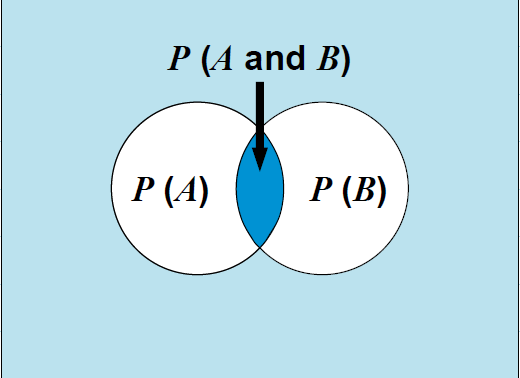
P (A|B) = P(A) + P(B) - P(A and B)

Statistically Independent Events

The occurence of one event has no effect on the probability of occurence of the second event.

Example:

• Snow in Santiago, Chile

• Rain in Tel Aviv, Israel

1. Marginal

2. Joint

3. Conditional

Types of Probabilities

Marginal (or simple) Probability

is the probability of a single event occuring

Joint Probability (Independent Event)

is the probability of two or more events occuring and is equal to the product of their marginal probabilities for independent events

P(AB) = P(A) x P(B)

Conditional Probability (Independent Event)

is the probability of event B given that event A has occured

P(B|A) = P(B) or P(A|B) = P(A)

Conditional (Dependent Event)

P(A|B) = P(AB) / P(B)

Joint (Dependent Event)

P(AB) = P(B|A) P(A)

1.Clearly define the problem at hand.

2.List the possible alternatives.

3.Identify the possible outcomes or states of nature.

4.List the payoff (typically profit) of each combination of alternatives and outcomes.

5.Select one of the mathematical decision theory models.

6.Apply the model and make your decision.

6 Steps in Decision Making

Decisiom Making Under Certainy

The decion maker knowns with certainty the consequences of every alternative or decision choice

Decision Making Under Uncertainty

The decision maker does not know the probabilities of the various outcomes.

Decision Making Under Risk

The decision maker knows the probabilities o the various outcoems

1. Maximax

2. Maximin

3. Criterion of Realism (Hurwicz)

4. Equally Likely (Laplace)

5. Minimax Regret

What are the criterias for making decisions under uncertainty?

Maximax

Used to find the alternative that maximizes the maximum payoff

Maximin

Used to find the alternative that maximizes the minimum payoff

Criterion of Realism

is a weighted average compromise between optimism and pessimism

• value of 0 is perfectly pessimistic

• value of 1 is perfectly optimistic

Weighted average =  a(maximum in row) + (1 – a)(minimum in row)

Equally Likely (Laplace)

Considers all the payoffs for each average. (Find the average, select the highest avereage)

Minimax Regret

Based on opportunity loss or regret, this is the difference between the optimal profit and actual payoff for a decision.

Decision Making Under Risk

This is decision making when there are several possible states of nature, and the probabilities associated with each possible state are known.

Expected Monetary value (EMV)

most popular method is to choose the alternative with the highest —

payoff of first state (probability) + payoff of 2nd state (probability)…

Expected Value of Perfect Information (EVPI)

• places an upper bound on what you should pay for additional information

• is the long run average return if we have perfect infromation before a decision is made.

(EVPI = EVwPI - Maximum EMV)

Expected Opportunity Loss (EOL)

• is the cost of not picking the best solution

• Minimum — will always result in the same decision as max EMV

Sensitivity Analysis

examines how the decision might change with different input data.

Decision Trees

• a graphical representation of a decision table

• are most beneficial when a sequen of decsions must be made

• contain decision points or nodes from which one of several alternatives may be chosen

• contain state-of-nature points or nodes, out of which one state of nature will occur

Structure of Decision Trees

• Trees start from left to right.

• Trees represent decisions and outcomes in sequential order.

  • Squares represent decision nodes.

  • Circles represent states of nature nodes.

  • Lines or branches connect the decisions nodes and the states of nature.