Y2 Intermediate Microeconomics Semester 1 Key terms

Three Axioms of Consumer Preferences:

• Completeness

• Transitivity

• Monotonicity

Completeness Axiom of Consumer Preferences:

• Completeness

  • Consumers possess preferences over all possible bundles

  • Consumers prefer bundles or is indifferent between the two

Transitivity Axiom of Consumer Preferences:

• Transitivity:

  • consumer preferences are logical

    • A > B, B > C, A should be > C

    • indifference should be consistent

Monotonicity Axiom of Consumer Preferences:

• Non-Satiation / Monotonicity:

  • Any marginal increase in the quantity of a good generates an increase in consumer’s utility

  • more = better

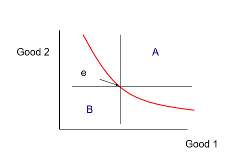
5 Properties of Indifference Curves

• Utility is increasing in the distance from origin

  • Non-satiation, consumer must prefer any point in A > bundle e (more area = more of good + distance from origin

• An indifference curve passes through every possible bundle

  • follows completeness ; consumer must be able to rank all bundles

• Cannot cross

  • crossing invalidates indifference as comparisons are now made

• Cannot have a positive gradient

  • bundle higher on the IC has more of at least one good and must be preferred rather than being indifferent.

• Cannot be took thick

  • if a curve is more than one bundle thick, we can pick a point that has 1+ good compared to another point and is thus preferred, following from non-satiation

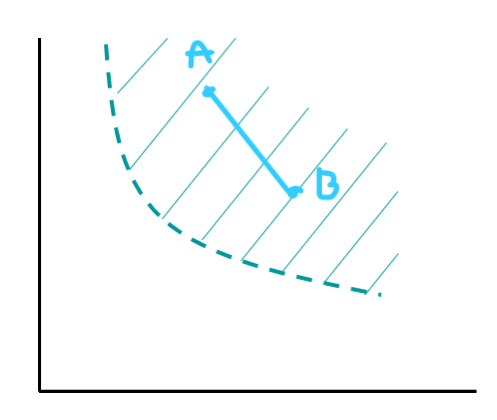
A common property of “Standard” Indifference Curves”

• Very commonly convex to the origin

  • if you shade area above curve, any two points within can be connected without leaving the area, and thus the weakly preferred set is convex

MRS and Indifference Curves:

Marginal Rate of Substitution (MRS)

• MRS - gradient of IC

• Maximum amount of one good that the consumer would be willing to sacrifice in order to obtain one more unit of another good.

  • e.g. MRS = -2. ; willing to give up 2x Y for +1 X

• MRS is diminishing due to gradient on standard ICs

• Consumers prefer mixtures of goods according to convexity, rather than extremes

Utility functions and IC:

• value of utility functions only tell us if A > B, cannot quantify by how much.

  • U(A) = 10 > 1 = U(B) and U(A) = 150 > 133 = U(B)

  • Both mean exactly the same thing: A is preferred to B

• U (X,Y) = 3X+5Y , V (X,Y) = 8+6X+10Y

• For (1,2) vs (2,1):

  • U(1,2) = 13 > 11 = U(2,1) ; (3)(1) + (5)(2) = 13 etc.

  • V(1,2) = 34 > 30 = V(2,1)

Utility functions and Monotonic transformations:

• U (X,Y) = 3X+5Y , V (X,Y) = 8+6X+10Y

• For (1,2) vs (2,1):

  • U(1,2) = 13 > 11 = U(2,1) ; (3)(1) + (5)(2) = 13 etc.

  • V(1,2) = 34 > 30 = V(2,1)

• Monotonic transformations:

  • If V (X,Y) = 2U (X,Y) + 8, rankings are unchanged

  • involve taking the square root of U(X,Y) , e.g. V(X,Y)= √(U(X,Y)

    • or its logarithm, e.g. V(X,Y)= ln (U(X,Y)).

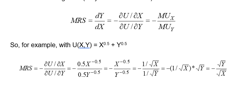
Mathematics for marginal utilities for two goods: 

• equation is a cobb douglas function

• partial derivatives are first time (0.5 and take away 0.5 to X is now denominator)

• Solve equation

• If X is large relative to Y, the MRS is smaller meaning the consumer is willing to give up less Y to get an extra unit of X.

• If Y is large relative to X, the MRS is larger , meaning the consumer is willing to give up more Y for X.

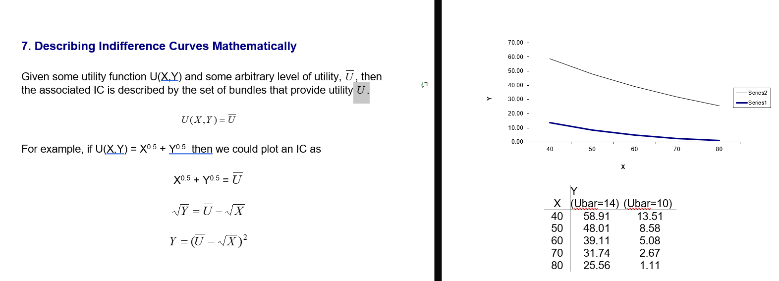
How to mathematically represent and calculate indifference curves:

• determine function

• Rearrange to have Y as subject

• Divide both sides by square root to get just Y

• plot and draw IC

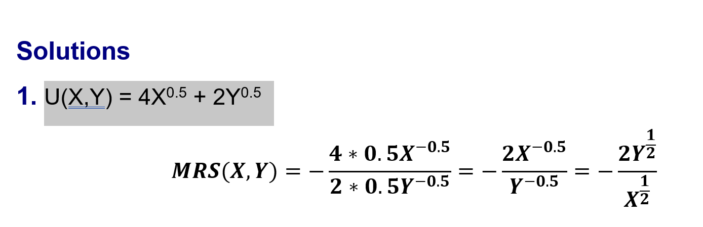
how to find MRS of utility function:

1. U (X,Y) = 4X^0.5 + 2Y^0.5

(negative because of formula above)

Step 1 - bring down power and subtract 1

• MRS (X,Y) = - 4 0.5X^-0.5 / 2 0.5Y^-0.5

Solve:

• MRS = - 2x^-0.5 / Y^-0.5

Step 2 - flip powers to positive but fractions flips too

Therefore, = - 2Y^1/2 / X^1/2

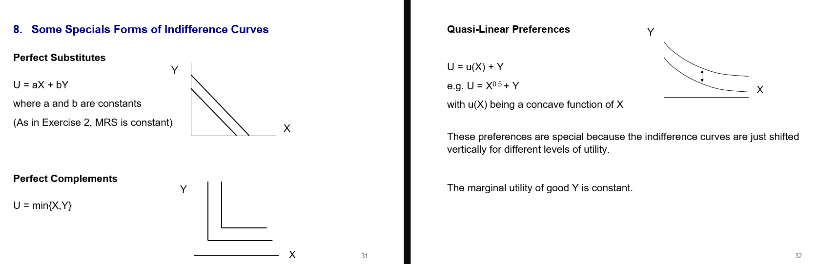
3 types of special indifference curves 

• Perfect substitutes

  • U = aX + bY

• Perfect complements

  • U = min (X,Y)

• Quasi-Linear Preferences

  • U = u(X) + Y such as X^0.5

    • u(X) a concave function of X

    • Marginal utility of good Y is constant

How to construct a demand function as part of demand and elasticity:

Constructing a demand function

• We want to find the DF for good H, as a general function of pg, ph and M; H* = H* (pg,ph,M)

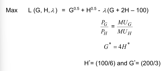
Add budget constraint

1. Max U (G,H) = G^0.5 + H^0.5 st. pgG + phH = M

Rearrange

1. Max U (G,H) = G^0.5 + H^0.5 - λ (pgG + phH - M)

Partial diffs

1. ∂L / ∂G = 0.5G^-0.5 - λ pg = 0

2. ∂L / ∂H = 0.5H6-0.5 - λ ph = 0

3. ∂L / ∂λ = -(pgG + phH - M) = 0

Equate to remove lamda, then rearrange to find optimal ratio

1. 0.5G^-0.5 / 0.5H^-0.5 = Pg / ph

2. ph / SQRT’G’ = pg / SQRT’h

3. G* = (ph^2 / pg^2)H*

Insert optimal ratio into BC

1. G* = (ph^2 / pg^2)H* with pgG* + phH* = M

2. pg [(ph^2 / pg^2)H*] + phH* = M ; converge and rearrange

3. (ph^2 / pg)H* + phH* = M

4. H* ((ph^2 / pg) = ph) = M ; remove H from each of the values*

5. H* = M / (Ph^2 / pg) + ph

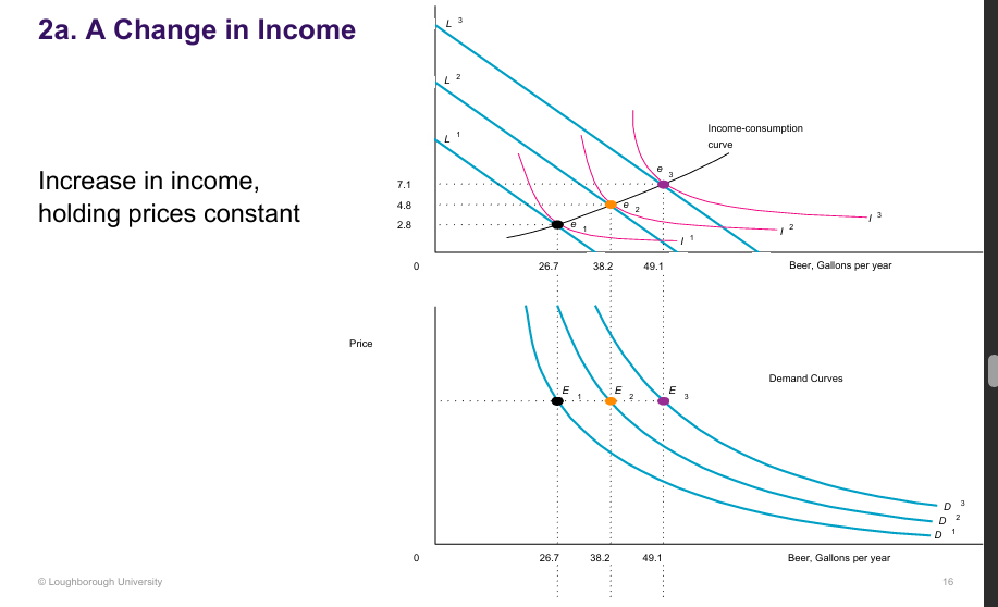
Change in income for Comparative Statics:

• Consumption increases as income rises; the DF defines inferior and normal goods

If ∂H*/∂M > 0 ; Good H is a normal good.

If ∂H*/∂M < 0 ; Good H is an inferior good.

e.g. public transport, having children = inferior good

Our example before, we can verifying that good H is a normal good

H = M / (ph^2 / pg) + pH*

Comparative statics:

Comparative statics

• A change in ENV will affect consumer behaviour

• Gov - taxation, spending, regulation, policy decisions

• Firm - pricing, marketing, investment decisions

• Comparative statistics: analysis of changes in EQ that occur due to Env changes.

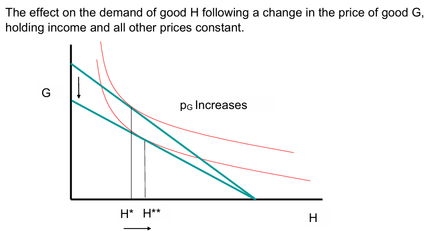
Change in Different’s good Price of Comparative Statics: 

• Price of good G increases → The budget line pivots inwards, since G becomes relatively more expensive.

• Substitution effect → Consumers substitute away from the now pricier good G toward good H, increasing demand for H from H* to H**.

• Income effect → The rise in pGp_GpG reduces real purchasing power, slightly offsetting the substitution effect depending on whether H is normal or inferior.

• Goods G and H are substitutes (∂H/∂pG > 0)*

If ∂H/∂pG > 0 ; Good G and good H are substitutes (coke and pepsi)*

If ∂H/∂pG < 0 ; Good G and good H are complements (cars + petrol)*

If ∂H/∂pG = 0 ; Good G and good H are independent goods (choc + hats)*

Change in Income of Comparative Statics:

• Consumption increases as income rises; the DF defines inferior and normal goods

If ∂H*/∂M > 0 ; Good H is a normal good.

If ∂H*/∂M < 0 ; Good H is an inferior good.

e.g. public transport, having children = inferior good

Our example before, we can verifying that good H is a normal go

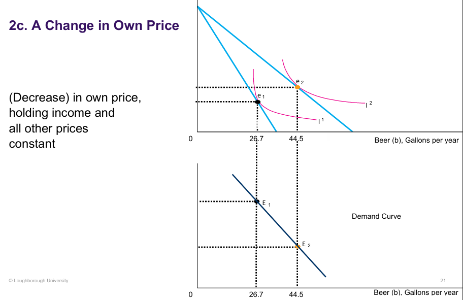
Change in Own Price of Comparative Statics:

Own price of beer decreases → The budget line pivots outward, allowing the consumer to buy more beer with the same income.

• New equilibrium → Consumption moves from e₁ to e₂ as the consumer reaches a higher indifference curve.

• Demand curve → The bottom graph shows that as the price falls, the quantity demanded increases — law of demand.

If ∂H/∂pH < 0 ; Good H is an ordinary good.*

If ∂H/∂pH > 0 ;Good H is a Giffen good*

Income elasticity of demand: 

• % change in demand for good H that follows 1% increase in income

  • A good is normal following ∂H/∂M > 0 ,* positive income elasticity because n>0 (M/H*>0)

n = % change in H / % change in M = ∂H/H / ∂M/M = ∂H* / ∂M x M / H****

Cross elasticity of demand:

XED: (for good H) % change in demand for good H that follows a 1% increase in the price of good G

𝜀𝐻G = % change in H / % change in pg = ∂H / ∂pg x pg / h***

• Goods G and H will have positive XED if substitutes and negative XED if complements (negative = opposite action e.g. price increase leads to demand decrease and vice versa)

• 10% increase in cigarette price —> low income families reduce food demand by 17%

  • substitutes as LYF substitute food for ST cigarette satisfaction on a low budget

Demand function context - You own a business producing training shoes. Using past data, you estimate the demand for your product. The results suggest that your monthly sales, Qi, can be expressed by the following, where M is average income, {pA, pB, pC} are the prices of other firms and pi is your own price.

Qi = 0.6M + 0.7pA + 0.3pB - 0.2pC – 0.6pi

Qi = 0.6M + 0.7pA + 0.3pB - 0.2pC – 0.6pi

0.7PA = substitute (higher coefficient —> higher substitutability); higher PA increases sales

0.3PB = weak substitute

0.2PC = weak complement

Closest rival = Firm A; price has largest positive coefficient (0.7)

• My sales respond most strongly to changes in Firm’s A price

Q) Currently, your price is 10, average income is 700 and your sales are 50. If income rises by 1% and price rises by 1%, what % change do you expect in your sales? (Hint: find the value of the income elasticity under these conditions).

Income elasticity: EM = 0.6 x 700 / 50 = 8.4 ; EM = M x Average Income / Sales

• 1% rise in income —> 8.4% increase in sales

Price elasticity: Ep = -0.6pi x 10 / 50 = -0.12 ; Ep = pi x price / sales

• 1% increase in price —> 0.12% reduction in sales

From econometric analysis, you know the sales of whiskey, QW, can be expressed by the following, where M is average income, and pW is the price of whiskey.

QW = 100 – 0.1M – 0.2pW

Currently, the price of whiskey is 10, and sales are 40. You are asked to predict the % change in whiskey sales after a potential tax increase that would lead to a 1% increase in the price of whiskey. Verify that your prediction would be -0.05%.

pw = 10

Qw = 40

Step 1 - FInd PED

1. Epw = dQw / dPw x Pw / Qw

2. dQw / dPw = -0.2 (in Equation)

3. Epw = (-0.2) x pw/qw = (-0.2) x 10/40 = - 0.05

Therefore, 1% increase in price —> -0.05% decrease in whiskey sales after a potential tax increase