ECON 201 - Drexel University Midterm 2 Review

When the price of one good rises...demand

decreases

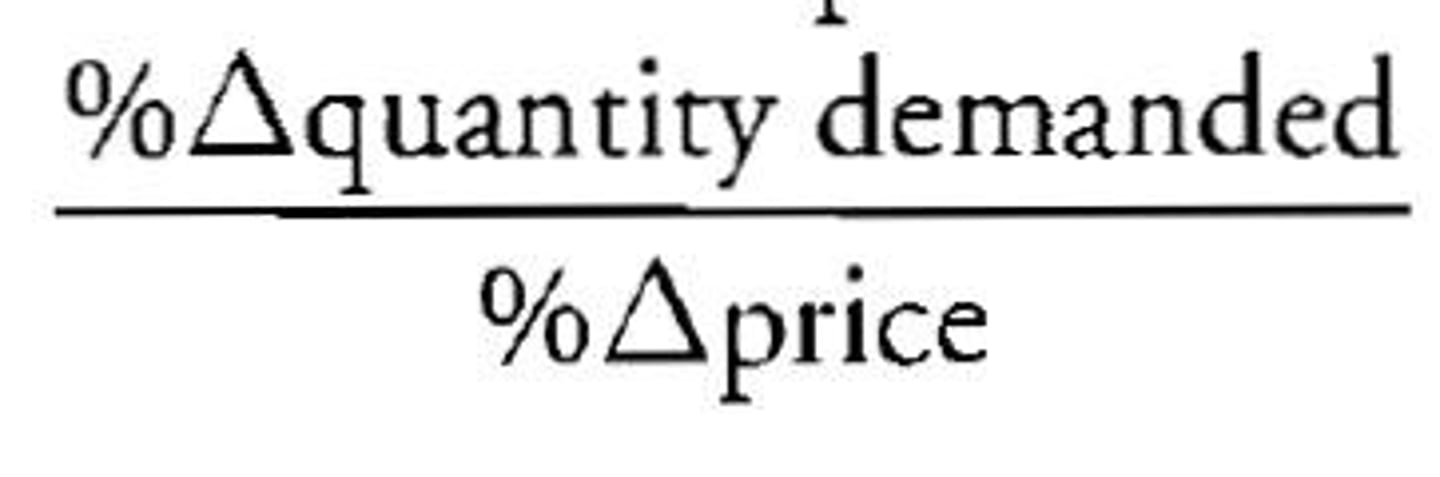
price elasticity of demand

the percentage change in quantity of the demanded good by that results from a 1% change in price

elastic

the demand for the good is elastic with respect to price if its price of elasticity is greater than 1

inelastic

the demand for the good is inelastic with respect to price of elasticity of demand is less than 1

unit elastic

the demand for the good is unit elastic with respect to price if its price elasticity of demand equals 1

elasticity

used as a measure of the extend of the response of either quantity demanded or supplied

Formulas for elasticity

E(Y,X) = % change in Y/% change in X

= %∆Y/%∆X =

=∆Y/Y / ∆X/X =

= ∆Y/∆X* X/Y

(own-) price elasticity of demand

measures the percentage change in the quantity demanded that results from a one percent change in its price

Ordinary good

Normal good

(elasticity > 0)

Luxury /Superior good

(elasticity > 1)

Necessary good

(elasticity <1)

Giffen good

Inferior Good

(elasticity < 0)

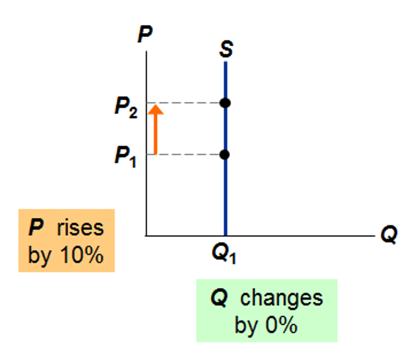
perfect elastic

if its price of elasticity of demand is infinite along a horizontal demand curve

ex. Pepsi (v.s Coca-Cola)

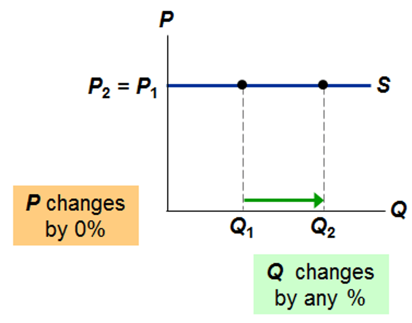
perfectly inelastic

with respect to price if its price elasticity of demand zero at every point along the demand curve

ex. Insulin

the flatter the demand curve

the more elastic is demand

steeper the demand curve

the less elastic is demand

∆Q/∆P

slope

consumer expenditures/producer revenue

change with changes in prices

Consumer Expenditures

= P*Q= Total revenues

P

price

Q

quantity

if the price elasticity of demand is less than 1

changes in price and changes in total revenue always move in the same direction

if the price elasticity of demand is greater than 1

changes in price and changes in total revenue always move in opposite directions

If demand is...

elastic

with a price increase will...

reduce total expenditure

^P * vQ = v PQ

If demand is...

elastic

with a price reduction will...

increase total expenditure

vP * ^Q = ^ PQ

If demand is...

inelastic

with a price increase will...

increase total expenditure

^P * vQ = ^ PQ

If demand is...

inelastic

with a price decrease will...

reduce total expenditure

vP * ^Q = v PQ

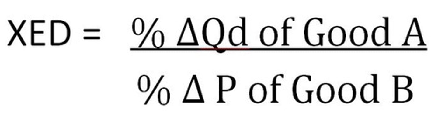
cross-price elasticity of demand

defined as the percentage change in quantity demanded of good A from a 1 percent change in the price of good B

Negative cross-price elasticity

complements

positive cross-price elasticity

substitutes

income elasticity of demand

defined as the percentage change in quantity demanded form a 1 percent change in income

positive income elasticity

normal good

negative income elasticity

inferior good

Perfectly Competitive Supply

MB ≥ MC

sellers will want to sell one more unit of output so long as their additional benefit from doing so exceeds their additional costs (explicit and implicit)

Additional cost to producing an additional unit

measured as the marginal opportunity cost

market supply curve

describes the quantity supplied at any given price summed up across all individual sellers in the market

reservation price

the maximum price a consumer is willing to pay for a product or service based on the total perceived consumer benefits

economic profit

difference between a firm's total revenue and the sum of its explicit and implicit costs

- also called excess profits

ex. market price multiplied by the number of units sold minus all costs (explicit and implicit)

profit-maximizing firm

one whose primary goal is to maximize the difference between its total revenues and total costs

perfectly competitive market

one in which no individual supplier has any significant influence on the market price of the product

price takers

firms operating in a perfectly competitive market

- take market price as given and chooses production level according

Perfectly Competitive Market Factors

1) Standardized Products

- identical goods offered by many sellers

- no loyalty to your supplier

2) Mobile Resources

- inputs move to their highest value use

- firms enter and leave industries

3) Many Buyers, Many Sellers

- each has small market share

- no buyer or seller can influence price

- price takers

4) Informed Buyers and Sellers

- buyers know market prices

- sellers know all opportunities and technologies

imperfectly competitive

a market in which individual firms are able to affect market prices

price setters

firms that have the ability to manipulate market prices through their choice of output

Examples of imperfectly competitive and price setters

= markets with relatively few firms (typically)

ex. commercial aircraft, microprocessors, electronics, electricity, cable, etc.

A factor of production

input used in the process of producing a good or serivice

Ex. Barber shop

Capital (K): scissors, razors, combs, chairs, etc.

Labor (L): barber

fixed factor of production

input whose quantity cannot be altered over the short term

ex. in the short run

coal mining equipment

ex. can't move a school, change mascot, etc.

variable factor of production

input whose quantity can be varied or altered in the short run

ex. coal miners

ex. teaching assistants at the school

law of diminishing returns

as output increases beyond some point, additional output gains associated with employing additional factors inputs begins to diminish

Four Kinds of Costs

Fixed Cost (FC)

Variable Cost (VC)

Total Cost (TC)

Marginal Cost (MC)

sunk cost

fixed cost

ex. lease payment price

Fixed Cost

sum of all payments made to the firms fixed factors of production. It does not depend on the number of things the firm makes

FC = rK

(rental rate*capital)

Variable Cost

company's payments to employees - vary with the number of things the firm produces

price of labor as wage (w)

VC = wL

Total Cost

sum of fixed and variable costs

TC = FC + VC

TC = rK + wL

Marginal Cost

the change in the total cost divided by the corresponding change in output

MC = ∆TC/∆Q = ∆VC/∆Q

Profits

total revenue - total costs

( P * Q ) - ( FC + VC )

profit maximization

so long as the additional revenue from producing one additional unit of output exceeds the additional cost of production, the firm's best option is to keep expanding output

MR≥MC

Competitive firm's rule for choosing the profit-maximizing output level

P=MC

Firm Shut Down Conditions

When certain costs are unavoidable (sunk) in the short term (ex. leased aircraft), firms are better off continuing to produce (at the profit maximizing level) as long as they can cover all of their variable costs (VC), plus a portion of their fixed costs (FC)

Short-Run-Shut-Down Rule

Cease production if TR=P*Q < VC for every level of Q

Average variable cost (AVC)

VC/Q

P< VC/Q = AVC

Profit is equal to...

(profit maximization)

(P-ATC)*Q

"Law" of Supply

- short-run marginal cost curves have a positive slope (higher prices generally increase quantity supplied)

- in the long run, all inputs are variable (Long-run supply curves can be flat, upward sloping, or downward sloping)

- perfectly competitive firm's supply curve is its marginal cost curve (at every quantity on the market supply curve, price is equal to the seller's marginal cost of production; applies in both short and long run)

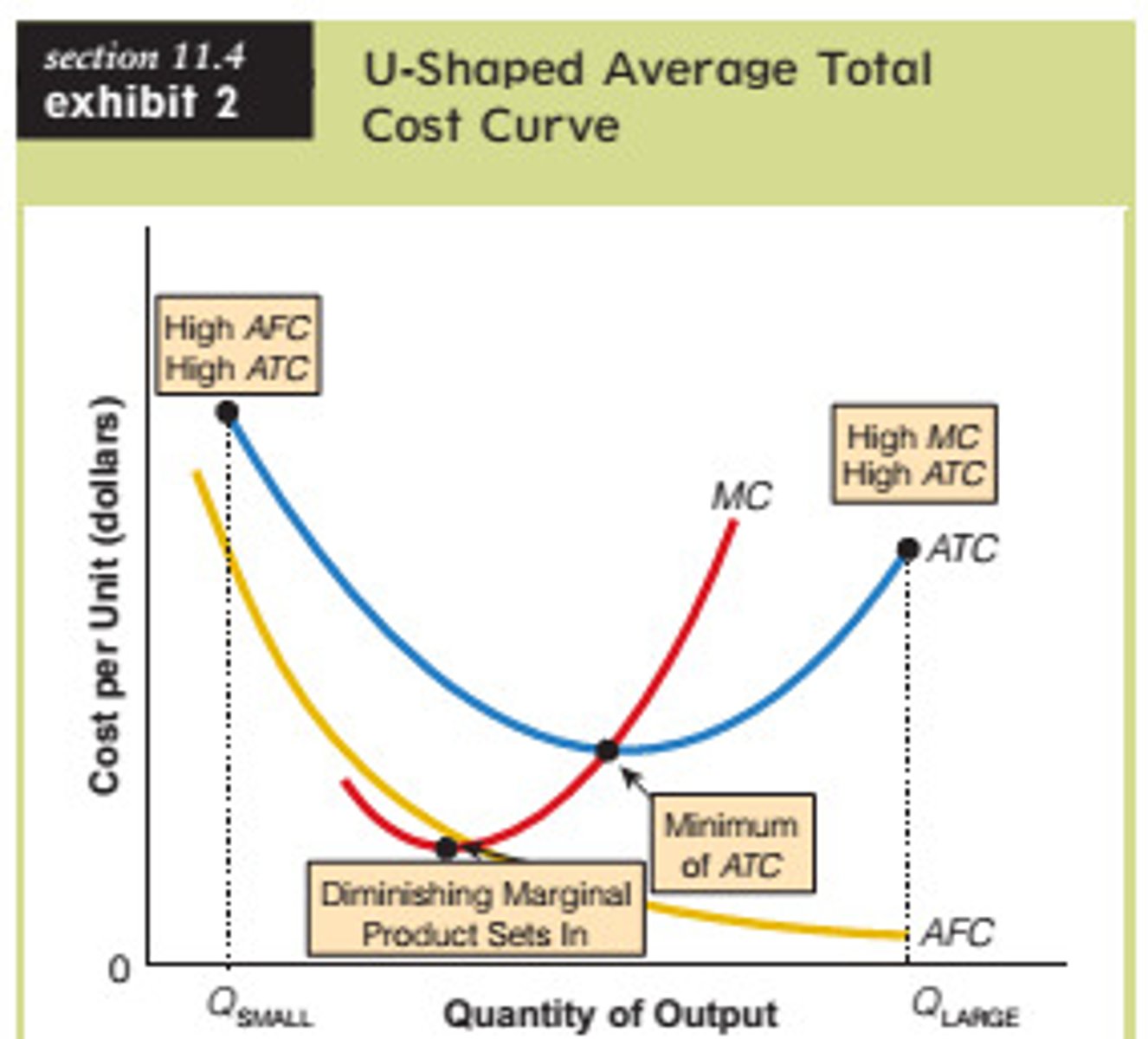
Marginal Cost Curve

a graphical representation showing how the cost of producing one more unit depends on the quantity that has already been produced

Average Variable Cost Curve

never crosses the average total cost curve.

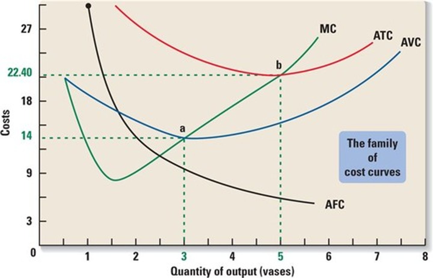
Average Total Cost Curve

shows the relationships between ATC and qty produced. at small production quantities, the ATC are high, with more production, costs decrease then eventually rise. the vertical sum of AVC and AFC

market dynamics

every time you see one of these signs

- Store for Lease

- Going out of business

- Now open

- close-out model

- under new management

The Invisible Hand

individuals act in their own interests

- aggregate outcome is collective well-being

Profit motive

- produces highly values goods and services

- allocates resources to their highest value use

(Lebron James doesn't not wait tables)

Accounting Profit

total revenue - explicit costs

- easy to compute

- easy to compare across firms

Explicit costs

payments firms make to purchase

- resources (labor, land, etc.) and

- products from other firms

implicit costs

the opportunity costs of the resources supplied by the firm's owners

normal profit

the difference between accounting profit and economic profit

- normal profits keep the resources in their current use

Person X earns about $10,000. C has an accounting profit of $15,000. Should X keep his job or open his own business?

open your own store, he has $5,000 extra. Take in OC

Economic Profit

= Accounting profit - normal profit

Rationing function

price distributes scarce goods to consumers who value them most highly

Allocative function

price directs resources away from overcrowded markets to markets that are underserved

Invisible Hand Theory

states that the actions of independent, self-interested buyers and sellers will often result in the most efficient allocation of resources

Responses to Profits and Losses

-Firms that earn normal profit recover only their opportunity cost

-firms that earn positive economic profit recover more than their opportunity cost

- markets in which firms are earning economic profit will attract resources

- markets in which firms are suffering economic losses will lose resources

Markets with excess profits attract resources

market price, standard supply and demand

- standard economic profit

Markets with supply increase

- lower market price

- supply shift to the right

- smaller economic profit

markets with zero economic profits

- smaller market price than with supply

- no economic profit

markets with resources leave

- smaller market price than zero economic profits

- negative economic profit