Linear Modelling

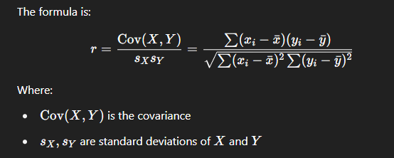
Correlation vs Causation

Correlation:

• Linear association between 2 variables

• Ranges from -1 to +1

• Correlation does not imply causation

Causation:

• One variable directly affects another

Correlation Formula

What is a linear model

Expresses relationship between a response (dependent variable) “y” and one or more predictors “x1”, “x2”

Estimates average change in “y” for a one unit change in a predictor, holding other variables constant

Why do we include an error term?

1. To account for natural variability in data

2. To capture effects of variables not included in model

3. To show predictions won’t be exact

4. Follows null distribution: ϵi∼N(0,σ2) to make it easier to infer

Model Assumptions

• Linearity: Relationship between predictors and response is linear.

• Independence: Residuals are independent.

• Homoscedasticity: Residuals have constant variance.

• Normality of residuals: Residuals are normally distributed.

• Mean of residuals = 0.

Goal of Modelling

• To understand relationship between different variables

• Once we know the relationship we can use the model to make predictions

Broom Package

Takes messy output of built-in-functions in R (Eg. lm) and turns them into tidy data frames

Functions

Represents the relationship between an input/s and an output.

How to find predicted values

Only consider x values that are within of the x value that you have used to estimate the model.

Eg. If data ranges from x=50 to x=100, don’t use model to predict for x=150.

The model might not hold for values outside the observed data

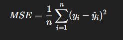
Mean Squared Error (MSE)

Measures how close the fitted model(line of best fit) is to the actual model and ensures its as close as possible.

Find average of squared differences between observed values (yi) and predict values(y hat)

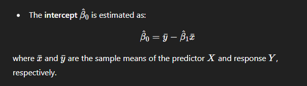
Coefficient B0:

Intercept.

When all variables are 0, what is the value of y

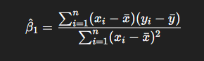
Coefficient: B1

Slope

• Measures expected change in y when x increases by 1 unit.

Alternate Formula:

Cov(x,y) / Var(x)

Visualising Residuals

Plots:

1. Residual Plot

2. Index Plot

3. Q-Q Plot

4. Histogram

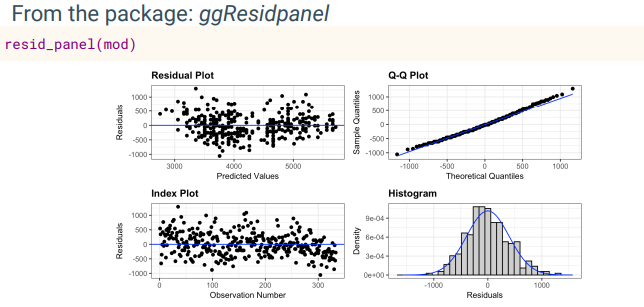
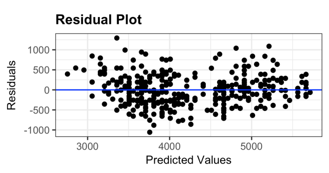
Residual Plot

• Shows residuals vs predictions

• Residuals should fluctuate around 0 with no pattern

• If there’s a pattern with residuals → indicates non-linearity (the linear model doesnt fit the data well

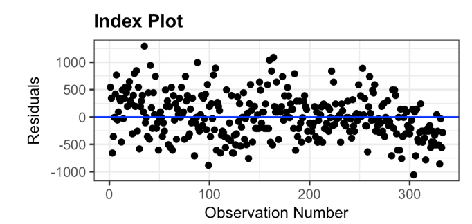
Index Plot

• Shows residuals vs observations

• Residuals should randomly fluctuate around 0

• If there’s a pattern, this shows autocorrelation (residuals are not independent)

• Autocorrelation is bad and violates assumption of independent errors

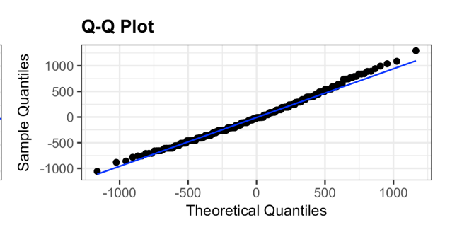
Q-Q Plot

• Compared model vs normal quantiles

• Useful for checking normal distribution assumption

• Should be a straight diagonal line if residuals are normally distributed

• Large deviation from the line indicate non-normal residuals which violates assumption of model

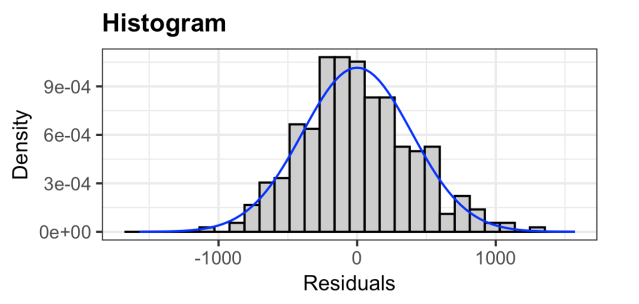
Histogram

• Bar plot showing frequency of residuals

• Should be bell shaped and symmetric (normally distributed)

• Checks normality assumption (Similar to Q-Q Plot)

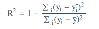
R² (Coefficient of determination)

R² = SSE/SST

R² = 1- (SSR/SST)

Ratio between explained variance and total variance

Tells us % of total variability in dependent variable that is explained by model

• Between 0 and 1 (1 = perfect fit)

• Adding more variables does not decrease R² but it might increase (even if variables are not useful)

R² vs Adjusted R²

Adjusted R² takes model complexity into account

More variables increase model complexity

Adjusted R² penalises adding unnecessary predictors

Dummy Variable

Categorical variables are shown as dummy variables

Intercept = Mean outcome for baseline category

Coefficients = Difference in response variable and baseline

Why should we do EDA before modelling?

• Helps understand data structure and spot patterns or problems (eg. missing values, outliers)

• Shows which model is appropriate to use

What can models show?

• Can show patterns not obvious in summaries

• However, can only show patterns that aren’t fully true leading to misinterpretation

Why should we check assumptions and residuals

• To make sure model is appropriate and not misleading

• Helps detect non-linearity, heteroscedasticity and autocorrelation

Goodness of fit measures

1. AIC

2. BIC

3. Deviance

AIC (Akaike Information Criterion)

• Can be used to compare models

• Smaller AIC = Better model

BIC (Bayesian Information Criterion

• Best way to compare 2 models

• Lower BIC = Better model

• Penalises model complexity more heavily than AIC

Deviance

• Measures residual variation (SSR - how much isnt explained by model)

• Closer to 0 = Better fit

• Best used for comparing 2 models (model with lower deviance is better)

Why do we use “average” in interpretations

• Regression estimates the average effect of a predictor on the dependent variable

• Actual observations vary around this average due to random error