SL Exam

A predictive model is trained using a clinical dataset to determine whether a patient will or will not develop cardiovascular disease over a specific follow-up window.

1. What kind of learning problem is that? (1p)

• Statistical learning

• Supervised learning

• Unsupervised learning

• K-means clustering with K = 2

This is a Supervised Learning problem (and falls within the broader framework of Statistical Learning).

2. What kind of outcome variable is it? (1p)

Select one or more alternatives

• Quantitative

• Binary

• Categorical

The outcome variable is Binary and Categorical.

3. Suggest suitable methods/algorithms to analyze this data. (1p)

Select one or more alternatives

• Extreme gradient boosting

• Clustering using mona (MONothetic Analysis Clustering of Binary Variables)

• Hierarchical clustering with 2 clusters

• Linear regression with ridge penalty

• Logistic regression with LASSO

• Logistic Regression with LASSO regularized penalty

• Extreme Gradient Boosting (XGBoost)

Question 2 (Q2)

Suppose that we try out two different statistical classification methods on a target clinical dataset.

First, we implement a baseline Logistic Regression model and obtain an error rate of 20% on the training partition and 30% on the independent validation test partition.

Next, we implement a Classification and Regression Tree (CART) model and obtain an average overall error rate (averaged across both the training and test datasets combined) of 18%.

Based on these empirical results, which specific method should we prefer to use for the classification of new, unseen observations?

We should prefer the Logistic Regression model.

When choosing a model to classify new observations, the decision must be guided strictly by performance on the unseen validation test set, as training set performance reflects data memorization rather than generalization.

Average Error Rate = training error rate + test error rate / 2
0% = In extreme overfitting, the tree creates splits to memorize all observations in the training set driving the error rate down to 0.

Test Error = (0% + 36%) / 2 = 18% = 18*2 = 36%

Because the true test error of Logistic Regression (30%) is lower than the projected test error of the CART model (36%),

A large biomedical dataset contains continuous high-dimensional gene expression measurements obtained from thousands of individual cells without any clinical group labels.

1. Why is this an unsupervised learning problem?

This is an unsupervised learning problem because the dataset lacks an explicit target outcome variable (Y) or known class labels to guide, supervise, or correct the model training loop. The algorithm must rely entirely on analyzing the joint distribution and geometric proximity of the input features (X).

2. What types of patterns might be discovered?

The algorithm can discover:

• Natural groupings or clusters representing previously unclassified cell sub-phenotypes

• Unique tissue lineages

• Highly correlated gene co-expression networks where sets of genes scale together functionally

3. Why can results depend heavily on preprocessing selections?

Unsupervised learning distance are highly sensitive to differences in feature scaling, data normalization, and batch effects.

If raw expression parameters are not standardized, high-magnitude or highly volatile genes will dominate distance matrices, skewing cluster boundaries based on arbitrary units rather than biological variance.

4. Why can interpretations of these low-dimensional configurations be challenging?

Unsupervised clustering and dimension reduction techniques identify purely mathematical relationships, geometric patterns, and spatial variance structures within the data grid.

These statistical groupings do not automatically translate into real-world or distinct biological functions, requiring independent experimental validation and domain-specific knowledge to interpret accurately.

A dataset contains gene expression from thousands of cells without labels.

Suggest a suitable method to discover patterns and groupings in this data.

Select one or more alternatives:

• Hierarchical clustering using diana (DIvisive ANAlysis Clustering)

• Linear regression if and only if the gene expressions are normalized, standardized and corrected for different batches

• Partitioning using PAM

• Extreme gradient boosting

• Hierarchical clustering using DIANA (Divisive Analysis Clustering)

• Partitioning Around Medoids (PAM)

Discuss how supervised and unsupervised learning differ in terms of:

1. Objectives

2. Availability of labels

3. Interpretation of results

4. Evaluation methods

1. Objectives

The primary objective of supervised learning is to construct a predictive map from input features (X) to a known outcome (Y), maximizing classification accuracy or minimizing regression residuals.

The primary objective of unsupervised learning is exploratory to uncover latent structures, natural groupings in input features (X) without a guiding target variable.

2. Availability of Labels

Supervised learning requires a complete, labeled training set where every observation vector is paired with a verified ground-truth outcome label.

Unsupervised learning operates entirely on unlabeled data configurations.

3. Interpretation of Results

Supervised interpretations focus on:

Directional slopes, Variable impact metrics, Feature importance, Explicit classification boundaries

Unsupervised interpretations focus on:

Spatial geometry, Cluster compactness, Structural co-expression profiles

4. Evaluation Methods

Supervised quality is calculated objectively via test performance metrics such as:

• RMSE

• AUC

• Sensitivity

• Specificity

These compare predictions against known test labels.

Unsupervised quality cannot use raw prediction errors, relying instead on:

• Cluster separation indices

• Silhouette widths (si)

• Internal validity measures

• Downstream biological validation

What are the different ways we can assess whether a trained statistical model will work reliably on new, unseen data?

1. Internal Validation Resampling Frameworks

This involves partitioning the baseline dataset to evaluate performance using:

• Train/test split

• k-fold cross-validation

• Repeated cross-validation

• Bootstrapping

These estimate out-of-sample error within a controlled framework.

2. External Validation Frameworks

This evaluates the final model on an entirely independent dataset collected from:

• A separate study population

• A different geographical region

• Another time period

This verifies true out-of-cohort generalizability

Can data splitting workflows yield unstable or highly misleading performance results?Select one or more alternatives:

• No, never

• Yes, a small validation set gives unstable performance estimates

• Yes, with an overall ‘small’ sample, splitting is inefficient (wasting data).

• No, we can impute stable results

• A small validation set gives unstable performance estimates.

• With an overall small sample size, splitting is inefficient because valuable data are withheld from model training.

A student is optimizing a predictive model pipeline.

(a) The student tunes the model's hyperparameters directly using the validation test dataset. Is this workflow problematic? If yes, why?

Yes, this workflow is highly problematic because it introduces data leakage.

By using the test set to choose hyperparameters, information from the test set leaks into the training loop. The test set is no longer a pristine, unbiased measure of generalized performance, leading to overly optimistic accuracy metrics that fail on truly new data

(b) Describe a better workflow for the scenario described in (a)

The original dataset should be partitioned into:

• Training set

• Test set

All hyperparameter tuning, feature engineering, and model selection decisions should be conducted solely within the training set using an internal validation strategy such as k-fold cross-validation.

Once the optimal hyperparameters are finalized, the model is fit on the full training set and evaluated exactly once on the untouched test set.

1. Explain what a hyperparameter is and outline the core purpose of conducting hyperparameter tuning.

A hyperparameter is an external configuration parameter set before the training process begins. Such as BMI, mean, median etc which is used to apply in the test data as a "recipe"

Examples:

• Lambda in LASSO/Ridge

• Tree depth

• mtry in Random Forest

The purpose of tuning is to find the value that minimizes test error by balancing the bias-variance trade-off.

2. Describe how the cross-validation framework can help identify a suitable model complexity level.

Cross-validation splits the training dataset into k equal segments (folds).

The model is repeatedly trained on k − 1 folds and evaluated on the remaining fold.

The average validation error across all folds is computed for each complexity level, producing a performance curve that identifies the complexity yielding the lowest expected test error.

A highly flexible machine learning model exhibits an exceptionally low training error rate but a high test error rate.

(a) Explain this specific performance configuration through the concepts of bias and variance.

This model is suffering from severe overfitting.

Its high flexibility minimizes bias but creates high variance.

Rather than learning only the true signal, the model has memorized noise and random fluctuations in the training data, causing poor performance on unseen data

(b) Explain the bias-variance trade-off principle clearly.

Expected test prediction error consists of:

• Squared Bias

• Variance

• Irreducible Error

As model flexibility increases:

• Bias decreases

• Variance increases

The goal is to find the level of complexity that minimizes the combined error.

(c) Suggest one concrete methodological strategy to reduce model variance

Variance can be reduced by simplifying model complexity, for example:

• Applying LASSO regularization

• Pruning deep decision trees

• Increasing sample size

• Using bagging or Random Forests

(a) What is bagging?

Bagging (Bootstrap Aggregation) is a variance-reduction ensemble technique that generates multiple independent training datasets by drawing random samples with replacement from the original dataset.

A separate model is trained on each bootstrap sample, and their predictions are combined using:

• Averaging (regression)

• Majority voting (classification)

(b) Explain how Random Forests utilize bagging.

Random Forests apply bagging by training many independent decision trees on separate bootstrap samples.

To further reduce variance and make trees less similar, only a random subset of predictors (mtry) is considered at each split.

This prevents a single dominant predictor from driving all tree structures and improves ensemble diversity

(c) Explain the core algorithmic idea behind boosting.

Boosting is an iterative ensemble method in which models are built sequentially rather than independently.

Each new model is trained to correct the residual errors or gradients left behind by the previously constructed ensemble.

(d) Why may boosted models overfit less than a single, deep decision tree?

A single deep tree can memorize noise and produce very high variance.

Boosting instead builds many small, shallow trees and combines them gradually using a learning-rate parameter (eta).

This allows the ensemble to learn complex patterns while reducing the tendency to overfit

(e) Why do ensemble methods often improve prediction performance noticeably?

Ensemble methods combine multiple diverse predictions.

This:

• Reduces variance (bagging)

• Corrects systematic errors (boosting)

As a result, they often achieve a better bias-variance balance than any single model.

(f) In bagging, all models contribute equally to the final prediction. How might we improve this approach if some models perform better than others?

This can be improved using:

• Weighted Ensembles

• Stacking (Stacked Generalization)

Rather than averaging predictions equally, a secondary meta-model learns how much weight each base model should receive, giving greater influence to more accurate models.

You have trained a predictive model that outputs continuous systolic blood pressure (mmHg) based on:

• Age (years)

• BMI (kg/m²)

• Plasma glucose (mmol/L)

The training cohort contains ages between 40 and 60 years only.

(a) You trained a linear regression model. Explain what happens if you apply it to individuals older than 60 years.

Linear regression will extrapolate beyond the observed data range.

Because the model assumes a constant age slope, it predicts that blood pressure continues increasing at the same rate beyond age 60.

If the true biological relationship changes, plateaus, or declines in older individuals, these predictions may become unrealistic.

You trained a Random Forest model. Explain what happens if you apply it to individuals older than 60 years.

Random Forests cannot extrapolate beyond the observed training range.

Individuals older than 60 will fall into the same terminal nodes as the oldest training observations.

Therefore, predictions tend to level off at a maximum value rather than continuing to increase indefinitely

1. Explain the purpose of regularized regression models (such as Ridge and LASSO).

Regularization reduces overfitting by adding a penalty on the size of regression coefficients.

Benefits include:

• Lower variance

• Better generalization

• Improved stability

• Better handling of multicollinearity

• Better performance when p > n

2. Explain the operational difference between Ridge and LASSO.

Ridge Regression

Uses an L2 penalty:

L2 Penalty = λ × Σ(βj²)

Effects:

• Shrinks coefficients toward zero

• Retains all predictors

• Does not perform variable selection

LASSO Regression

Uses an L1 penalty:

L1 Penalty = λ × Σ|βj|

Effects:

• Shrinks coefficients toward zero

• Can set coefficients exactly equal to zero

Performs automatic variable selection

3. Explain what happens when lambda (λ) increases

As λ increases:

• The penalty becomes stronger

• Coefficients are forced closer to zero

• Bias increases

• Variance decreases

Extreme cases:

λ → 0: Equivalent to ordinary least squares (OLS)

λ → ∞: Coefficients approach zero, leaving mainly the intercept term

A machine learning model predicts 5-year cardiovascular disease risk.

Performance on an independent test dataset:

• AUC = 0.91

• Sensitivity = 0.95

• Specificity = 0.55

Calibration analysis shows predicted risks are systematically too high for low-risk individuals.

 

1. Explain what the AUC value indicates.

An AUC of 0.91 indicates excellent discrimination.

It means there is a 91% probability that the model assigns a higher risk score to a randomly selected person who develops cardiovascular disease than to a randomly selected person who does not.

2. Interpret the sensitivity and specificity values.

Sensitivity = 0.95

• Correctly identifies 95% of true disease cases

• Produces few false negatives

Specificity = 0.55

• Correctly identifies 55% of healthy individuals

• Produces many false positives

Therefore, the model is much more likely to generate false alarms than miss disease cases.

3. Explain what poor calibration means. Why is calibration important?

Poor calibration means predicted probabilities do not match observed event frequencies.

For example, the model may predict risk levels that are consistently higher than reality.

Good calibration is important because risk estimates are often used directly in clinical decision-making.

Poor calibration may lead to unnecessary diagnostic testing

4. Discuss strengths and weaknesses of the model.

Strengths

• Excellent discrimination (AUC = 0.91)

• Very high sensitivity (0.95)

• Effective screening tool

Weaknesses

• Low specificity (0.55)

• Many false positives

• Overestimates risk among low-risk individuals

May increase unnecessary interventions

The following confusion matrix was obtained from an XGBoost model evaluated on a test dataset using a classification threshold of 0.5.

              Reference

Prediction     NO     YES

 

NO            262      36

YES           124    3077

Calculate PPV and NPV. Show all steps

Positive Predictive Value (PPV)

PPV measures the proportion of positive predictions that are correct.

PPV = TP / (TP + FP)

PPV = 3077 / (3077 + 124)

PPV = 3077 / 3201

PPV = 0.9613

PPV ≈ 96.1%

NPV measures the proportion of negative predictions that are correct.

NPV = TN / (TN + FN)

NPV = 262 / (262 + 36)

NPV = 262 / 298

NPV = 0.8792

NPV ≈ 87.9%

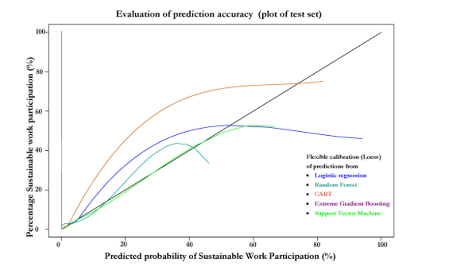
What does the plot show and how would you interpret the results?

The plot evaluates probability calibration.

• X-axis: Predicted probabilities

• Y-axis: Observed event frequencies

A perfectly calibrated model follows the 45-degree diagonal line.

Curves deviating from this line indicate overestimation or underestimation of true probabilities.

2. Which model would you choose if prediction performance and interpretability are weighted equally?

Logistic Regression

Reasons:

• Strong calibration

• Easy interpretation

• Coefficients can be converted into odds ratios

• Good balance between performance and transparency

Ten bootstrap samples produce the following estimated probabilities for:

P(Red | X)

0.10, 0.15, 0.20, 0.20, 0.55, 0.60, 0.60, 0.65, 0.70, 0.75

Classification threshold = 0.5

Green = 0
Red = 1

Determine the final prediction using:

1. Majority Vote

2. Average Probability

1. Majority Vote= Red (1)

2. Average Probability = Green (0)

(A) Explain one major limitation of clustering methods.

Clustering is an exploratory unsupervised method with no true outcome variable.

Therefore, there is usually no objective ground-truth error rate available for evaluation

(B) Why may different clustering methods produce different results on the same data?

Different clustering algorithms optimize different objectives.

Examples:

• K-means minimizes within-cluster variance.

• PAM minimizes dissimilarity to medoids.

• Hierarchical clustering uses linkage-based grouping.

As a result, they may produce different cluster structures.

(C) Give one example where clustering could be useful in genomics

Identifying previously unknown cellular subtypes from single-cell RNA sequencing data.

Which statements correctly describe the goals of cluster analysis?

Select one or more alternatives: To identify natural groupings in the data

To group observations into relatively homogeneous groups

To group observations that are similar to each other

To maximize differences within clusters

To minimize similarity between observations within the same cluster

To place observations with similar characteristics in the same cluster

To predict a nominal outcome variable

Correct Statements

• Identify natural groupings in the data.

• Group observations into relatively homogeneous groups.

• Group observations that are similar to each other.

• Place observations with similar characteristics into the same cluster.

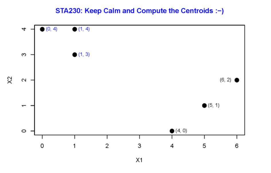
Compute the centroids

Left Centroid = (0.67, 3.67)
Right Centroid = (5, 1)

1. Explain why dimensionality reduction is useful

Dimensionality reduction compresses high-dimensional datasets into a smaller number of variables.

Benefits include:

• Noise reduction

• Reduced multicollinearity

• Improved visualization

• Faster computation

2. Explain the main goal of Principal Component Analysis (PCA).

PCA constructs orthogonal linear combinations of the original variables (principal components) that successively capture the greatest possible variance in the dataset.

3. Compare PCA with UMAP or t-SNE

Solution:

PCA

• Linear method

• Preserves global variance structure

• Fast and interpretable

t-SNE

• Nonlinear method

• Preserves local neighborhoods

• Excellent visualization tool

UMAP

• Nonlinear method

• Preserves both local and some global structure

Often faster and more scalable than t-SNE

4. Why are distances in t-SNE plots difficult to interpret?

t-SNE intentionally distorts global distances to preserve local neighborhoods.

As a result, distances between widely separated clusters are often arbitrary and should not be interpreted as meaningful measures of similarity.

5. Why are t-SNE and UMAP mainly used for visualization?

They compress complex high-dimensional datasets into 2D or 3D representations, making hidden structures, clusters, and patterns easier to visualize and explore.