Lecture 5 - PSYC3221

In the context of distance-dependent similarities in intensity values what does intensity and differences in intensities mean?

These distance-dependent similarities in intensity values imply that the distribution of luminance values (intensity) and differences in intensities (contrast) are scale dependent

Characteristics of spatial distribution of luminance variations in natural scenes

These distance-dependent similarities in intensity values imply that the distribution of luminance values (intensity) and differences in intensities (contrast) are scale dependent:

• At small distances (fine spatial scale, or local scale) the similarities in pixel intensities are likely to be high and differences are small (similar intensity, low contrast);

• At large distances (coarse spatial scale, or global scale) the similarities in pixel intensities are likely to be low and differences high (large differences in intensity; high contrast).

• One robust regularity is based on the spatial proximity between different image points or pixels in an image. The closer the points or pixels in an image are, the more similar in intensity they tend to be.

Spatial Scale Specific Intensity Variations in Natural Scenes at small and large distances

Spatial Scale Specific Intensity Variations in Natural Scenes:

Smaller distances:

• At smaller distances there is higher correlation in intensity between different points in an image; higher similarity in intensity between different points implies lower spatial contrast at smaller distances.

• We know that at smaller distances there is a high correlation between adjacent pixels in intensity. As a consequence, the contrast (or variations in intensity) within the red circled regions will be low

• When a natural scene is sampled by neurons with smaller receptive field size (like neurons sampling from the foveal region), it is likely that the receptive field centers and surrounds of these neurons will be simulated by similar intensities, or by small differences in intensity between the center and surround regions (low contrast)

• We can turn these red circular local regions in an image into concentric centre-surround regions, resembling the receptive field of neurons with small receptive field sizes

Larger distances:

• At greater distances there is lower correlation in intensity between different points in an image; lower similarity in intensity between different points implies higher spatial contrast associated with greater distances.

• Conversely, when a natural scene is sampled by neurons with large receptive field sizes (for example, neurons with receptive fields in periphery of the visual field), it is likely that they will be simulated by large differences in intensity between their centre and the surround regions.

Spatial Scale and Spatial frequency:

In vision, the spatial scale is usually referred to as spatial frequency;

• Low spatial frequency: intensity variations occur over a large spatial scale (large distances over space);

High spatial frequency: intensity variations occur over a small spatial scale (small distances over space);

what is meant by low and high spatial frequencies

In vision, the spatial scale is usually referred to as spatial frequency;

• Low spatial frequency: intensity variations occur over a large spatial scale (large distances over space);

• High spatial frequency: intensity variations occur over a small spatial scale (small distances over space);

where in the spatial frequency space is human peak Sensitivity? Contrast Sensitivity Function

Spatial Frequency Content and Visual Sensitivity: Contrast Sensitivity Function:

• Peak Sensitivity at intermediate spatial frequency

• Peak sensitivity is somewhere around six cycles per degree of a visual angle

Spatial Frequency Ranges and the Information they Convey

• Different spatial frequencies convey different information about the appearance of a stimulus. High spatial frequencies represent abrupt spatial changes in the image (such as edges), and generally correspond to fine detail (left panel). Low spatial frequencies, on the other hand, represent coarse variations in intensity over an image.

  • Low spatial frequency is sampled with neurons with large receptive field sizes (periphery of the visual field), while high spatial frequency is sampled with neurons with small receptive field sizes (centre of the visual field).

What is a Amplitude spectrum slope and  the amplitude spectrum graph?

Amplitude spectrum slope

• The amplitude spectrum slope describes relative proportions of energy (amplitude of intensity variations) at large scale structure and fine detail in the entire spatial distribution of image intensities.

• This graph is known as the amplitude spectrum graph and it plots the amplitude of intensity variations as a function of spatial frequency components of an image. On the X axis is the spatial frequency and on the Y axis is the amplitude of intensity variations (contrast) at a given spatial frequency in a scene.

• To create this graph, an image is decomposed into different spatial frequency components (ranging from low to high) and the amplitude of variations (contrast) associated with different spatial frequencies is plotted as a function of spatial frequency.

• What we see is that low spatial frequencies in an image are associated with high amplitude of intensity variations (with high contrast) while the high spatial frequencies in an image are associated with much smaller amplitude of intensity variations (much smaller contrast).

• In all natural images, regardless of what they represent on the surface (beach, street, forest), the amplitude associated with different spatial frequencies in an image falls off from the low spatial frequency to the high spatial frequency.

• It is essentially an inverse linear relationship between the amplitude of intensity variations and a spatial frequency component of an image.

• This particular shape, this inverse linear relationship between amplitude and spatial frequency, is thought to be related to the so-called scale invariance of natural scenes, or the notion that approximately equivalent amount of spatial structure can be found as we zoom in and out between the coarse or fine spatial scales in an image, between low and high spatial frequencies.

• The notion of scale invariance is related to the notion of self-similarity, and to the notion of fractals.

Mathematical fractal vs statistical fractal

Mathematical fractal vs statistical fractal:

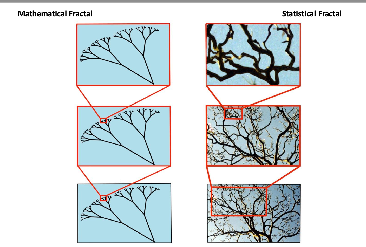
• In mathematical fractals the structure at different levels of magnification is exactly identical at every level of magnification and it can be extended inward or outward indefinitely.

• In nature, most fractals are statistical fractals, meaning that patterns at different levels of magnification are not identical, but only similar to each other.
  
  
  

What happens to an image as we change the slope of its amplitude spectrum?

• With the flattening, we are increasing the amplitude associated with high spatial frequency relative to the natural image and we are decreasing the amplitude associated with the low spatial frequency relative to the natural images → In a flattened amplitude spectrum, the amplitude associated with the low and high spatial frequency is more equalized and the modified image looks very much like a high spatial frequency filtered image.

• With the increased amplitude spectrum slope, we are even further increasing the amplitude that is associated with the low spatial frequencies compared to the natural scenes → We are also further decreasing the amplitudes associated with high spatial frequencies in an image.

Given that in natural scenes, the low spatial frequency has the higher contrast amplitude, low spatial frequency can be used to guide object identification and discrimination. The role of low spatial frequency components in visual system's ability to identify and differentiate between different objects has been confirmed in a study. What are the methods and results of this study.

• Given that in natural scenes, the low spatial frequency has the higher contrast amplitude, low spatial frequency can be used to guide object identification and discrimination.

• The role of low spatial frequency components in visual system's ability to identify and differentiate between different objects has been confirmed in a study by Goffaux and her colleagues from 2003:

• They were interested in the visual system's ability to differentiate between different classes of objects: faces and cars.

• They compared performance as well as EEG, electrophysiological. recordings of the brain activity in response to either full spectrum faces and objects, low spatial frequency faces and objects, and high spatial frequency faces and objects.

• Low spatial frequency component and high spatial frequency component were embedded in the noise of the complementary spatial frequency type, which is what is shown in these examples.

• As expected, here was a huge difference in brain response to faces and cars to full spectrum (unfiltered) images;

• The difference was just as big in response to just the low spatial frequency versions of faces and cars.

• The difference in activation pretty much disappeared for high spatial frequency versions of face and car images;

• These results were observed in the period between 160 and 220 milliseconds after onset of these images, showing that discrimination between faces and cars seems to be supported by low spatial frequency content of the image information

Even though high spatial frequency content of object images doesn't seem to be contributing very much to our visual system's ability to discriminate between different images, especially at early exposure, under unlimited viewing conditions, high spatial frequency can … What is the phenomenon of high spatial frequency masking?

Even though high spatial frequency content of object images doesn't seem to be contributing very much to our visual system's ability to discriminate between different images, especially at early exposure, under unlimited viewing conditions, high spatial frequency can overpower and mask the information conveyed by low spatial frequency in an image:

• This phenomenon is called high spatial frequency masking: Low spatial frequency information is hard to notice in the presence of high spatial frequency information. In this example, a light cross in this checkerboard pattern is hard to see with a high spatial frequency black grid superimposed over the checks. When the grid is removed (for example, by blurring it (which removes high spatial frequencies) —> eg., in pixelated images because the low spatial frequency component is being masked by the high spatial frequency of pixelated squares.

What is a hybrid image?

It is rather hard to disentangle separate contributions from low spatial frequency channels and high spatial frequency channels to the scene processing:

• A unique way to disentangle contributions from these different sources is through a special class of images called, hybrid images

• A hybrid image is a single picture that combines low spatial frequency information of one scene with high spatial frequency information from another scene. So essentially you have scenes with two different interpretations, one of which is conveyed in a low spatial frequency channel and the other is conveyed in high spatial frequency channel.

•  One thing that can be noticed immediately by inspecting these images and the images on the former slides is that under normal viewing conditions, high spatial frequency information seems to dominate interpretation of the hybrid image

The interpretation of hybrid images changes with the viewing distance. Which is more prominent at close and far distances?

The interpretation of hybrid images changes with the viewing distance:

• From a far distance, we will see primarily the low spatial frequency component

• From a closer view, we will primarily see the high spatial frequency component

• If the peak sensitivity is 6 cycles per degree, for this specific object, at this specific distance, the peak sensitivity is around 12 cycles per image.

• Size/distance dependent change of the interpretation of these images will happen in both cases.