Likharev Boxed Formulae Ch. 1-2

Coulomb law of force

k here is 1/4πε₀

Definition of the electric field

Electric field of a set of point charges

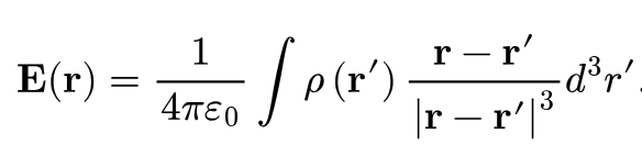
Electric field of continuous charge

Gauss’ electric field law

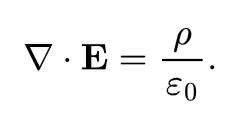
Inhomogenous Maxwell equation for electric field

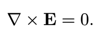
Homogeneous Maxwell equation for electric field

Definition of the electrostatic potential

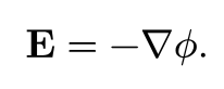
Electrostatic field expressed from potential

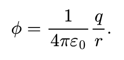
Electrostatic potential of a point charge

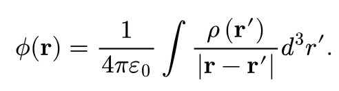
Electrostatic potential of continuous charge

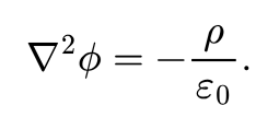
Poisson equation for electrostatic potential

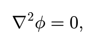
Laplace equation for electrostatic potential

A continuous charge’s energy in an external field

Interaction energy between two charges

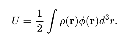
Energy of an electrostatic field

Spatial Green’s function for a point charge

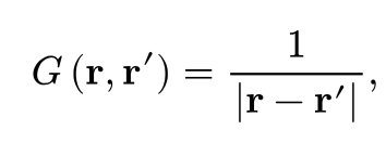
Does Green’s function for a point charge obey Poisson’s equation? How?

For a point charge, φ = (q/4πε₀) G(r, r’), this is a result of Green’s theorem.

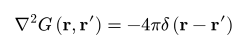
In electrodynamics, this is a condition required for all Green’s functions…

The Green’s functions vanish as soon as the radius vector r points to the surface (S) of any conductor!

Core relation describing the electric field screening effect

Inside the conductor, also φ = constant

Conductor surface charge density and normal electric field

Classical Debye screening length

Based on the assumption of a continuous charge distribution and charge carriers that obey Maxwell-Boltzmann statistics, this gives the length scale over which the electric field is screened by a conductor

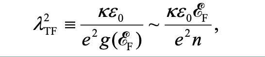
For very good metals, why does the Debye screening length break down and what is it replaced by?

Debye screening length is based on a Boltzmann distribution of charge which is not accurate for good metals, then you need to use Fermi-Dirac statistics with the density of quantum states and replace with the Thomas-Fermi screening length

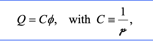
Self-capacitance of a conductor

Cursive p = proportionality constant which depends on the conductor’s size and shape and is often called the reciprocal capacitance

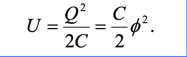
Electrostatic energy of a single conductor in terms of self-capacitance

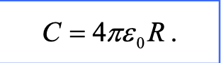
Self-capacitance of an isolated conducting sphere

A voltage between two conductors (total system is electrically neutral) describes

Difference in potential

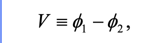
Mutual capacitance between two conductors when the total system is electrically neutral

These subscripts are wrong though, so like ρ₁ is really ρ₁₁ and ρ is ρ₁₂, these are elastances/reciprocal capacitances and you can make a matrix out of them typically, this formula emerges from the total system = neutral case

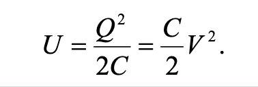
Electrostatic energy of a system of two conductors (capacitor)

System as a whole has to be electrically neutral though I think

Mutual capacitance of a parallel plate capacitor

When you cannot find the electric field in the space between two conductors via symmetry or Gauss’ law what should you use?

Laplace’s equation in between and the constant potential requirement on the surface of each conductor

Mutual capacitance per unit length of a coax

Mutual capacitance of a spherical capacitor

Laplace operator in cylindrical coordinates and the different solutions in separation of variables

AZIMUTH: solutions are Φ(φ) = A sin(mφ) + B cos(mφ) but this time m=0 or m>0 only, m=0 gives azimuthal symmetry, m>0 describes wedges held at alternating potentials

TRANSLATIONAL: when Z’’ = -k²Z you get Z(z) = A sin(kz) + B cos(kz), this describes a cylinder with grounded end-caps and gives standing waves along the length, when Z’’ = k²Z you get Z(z) = A sinh(kz) + B cosh(kz) and this describes an infinitely long cylinder or a cylinder with a non-grounded end-cap; when k = 0 you get either linear or constant Z (Az + B), when there is translational symmetry (aka infinitely long/uniform system) then A=0

RADIAL: you get ρ²R’’ + ρR’ + (+-k²ρ² - m²)R = 0; now this is the same k² so when Z(z) is exponential then R(ρ) = A J_m(kρ) + B Y_m(kρ), when Z(z) is oscillatory then you get R(ρ) = A I_m(kρ) + B K_m(kρ), when there is no z-dependence (translational symmetry) then k=0 and either m>0 (solutions become R(ρ)=A ρ^m + B ρ^-m) or m=0 (solutions become R(ρ) = A ln(ρ) + B)

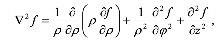
Laplace operator in spherical coordinates and the different solutions in separation of variables

AZIMUTH: m² gives Φ(φ) = A sin(mφ) + B cos(mφ); with azimuthal symmetry then m = 0, if boundary conditions involve vertical slices held at different voltages then m>0 and the potential needs to oscillate as you rotate.

POLAR: m and l(l+1) give summation of P^m_l (cos θ) the associated Legendre polynomials where l is an integer and -l <= m <= l (m also integer); with azimuthal symmetry then l=0 gives spherical symmetry & monopole, l=1 gives dipole, l=2 gives quadrupole

RADIAL: R(ρ) = Aρ^l + Bρ^-(l+1); decaying term is the field generated by a localized charge near the origin (l=0 gives monopole, l=1 gives dipole, etc) it gets thrown out if you include the origin. growing term represents an electric field imposed by external charges far away, it gets thrown out if you include out to infinity.

Laplace operator in rectilinear coordinates and the different solutions in separation of variables

k² > 0: exponential solutions f(x) = A sinh (kx) + B cosh (kx), used for the "open" dimensions of your geometry, if the region extends to infinity, you use the decaying exponential or a combo of both to get either 0 or some other value

k² < 0: oscillatory solutions f(x) = A sin (kx) + B cos (kx), if you have an enclosed space with two grounded surfaces facing each other you must use sines or cosines.

k² = 0: linear solution f(x) = Ax + B

In the spherical Laplacian solution, what is the physical insight tied to m and l? What are nodal lines?

A nodal line is where the potential is exactly zero. So the l index will give you the total number of nodal lines on the sphere, the m index will give you how many of them are LONGITUDINAL, and the l - |m| difference will give you how many of them are LATITUDINAL

What is this and what is it its solution?

This is the Bessel equation, and its solution cannot be satisfied by a single “elementary” function, you need to use Bessel functions.

Describe the behavior of J_m(kρ) and Y_m(kρ) at ρ=0 and ρ=infinity

Only J_m is finite at ρ=0. Both go to zero as ρ=infinity

Describe the behavior of I_m(kρ) and K_m(kρ) at ρ=0 and ρ=infinity

I_m grows exponentially as ρ—>infinity but it is finite at the origin. K_m goes to zero as ρ—>infinity but it blows up at the origin

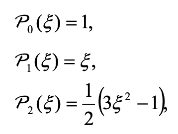
Rodrigues formula for the Legendre polynomials

First three Legendre polynomials

General solution to any axially symmetric spherical Laplace problem

General solution to any spherical Laplace problem

An arbitrary charge distribution creates the potential (include in terms of spatial Green’s function and both discrete/continuous case)….

What is the general solution for the potential φ given a volume charge distribution ρ(r’) and a system of bounding conductors held at potentials φ_k using the Dirichlet Green's function?"

Volume V does NOT include the conductors, the Green’s function in both integrals is the same and is the potential at r of a single point charge at r’ with the condition that G=0 on the surface of all the conductors

The cosine of the angle γ between the two position vectors r and r’ in spherical coordinates is…

When is it impossible to use method of images to find a Green’s function?

When there is some charge that is inside or on a conductor and no charge outside of it, that is when you cannot use method of images.

A Green's function calculates what the potential φ would be if your conductor contained absolutely nothing except one single, normalized point charge located at r’. You construct this tool completely blind to whatever actual charge ρ might exist in the prompt.

When you cannot use method of images to find a Green’s function, what do you need to use?

First, recall a Green’s function calculates the potential if the conductor only contains a single normalized point charge at r’. So first, you get the 3D dirac delta function of a point charge at r’ in your coordinate system. Then, you make an educated guess for G(r, r’) based on boundary conditions and the appropriate Double Fourier, Bessel Fourier, or Multipole/Spherical Harmonic expansions. You plug this into the Laplacian Green’s function equality which is del² G(r, r’) = - 4πδ(r-r’). You expand the 3D dirac delta in a symmetric way and then use orthogonality to cancel the summations. You should get a simpler differential equation.

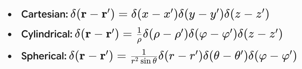
3D dirac delta in cartesian, cylindrical, spherical