Statistics 1: Definitions

Statistic

information from a sample (subset of a population)

Parameter

the summary of a population

Descriptive statistics

organizing and summarizing data (numerical summaries, tables, graphs, etc)

Inferential Statistics

take results from a sample (descriptive portion) and sees how applies to the population; measures reliability

Qualitative/Categorical variables

characteristics or attributes (not usually numerical)

Quantitative variables

numerical measures; can be added or subtracted

Discrete variable

countable, limited possibilities (ex: the number of students in a class, cannot be partial)

Continuous variables

continuous, infinite possible values, any level of accuracy (ex: height, weight)

Nominal level of measurement

the name of an item

Ordinal level of measurement

items are arranged in a specific order

Interval level of measurement

usually numerical, differences between items, addition or subtraction make sense, zero doesn’t mean the absence of quantity (ex: temperature)

Ratio level of measurement

accounts for factors, multiplication and division make sense, zero does mean the absence of quantity. (ex: speed)

Observational Study

observing a group of individuals (no intervention) over time and drawing a conclusion (ex: unethical studies)

Designed Experiment

organizing and manipulating a group of individuals and records the value of the response variable

Response variable

the response to the experiment (dependent variable)

Explanatory variable

what causes the response (independent variable)

Confounding

when the effects of two or more explanatory variables are not separated, so the result doesn’t imply causation in experiment

Confounding variable

an explanatory variable that cannot be separated from the independent variable but impacts experimental results

Lurking variables

not considered in a study but impacts the response

Simple random sampling

pre-determining the individuals that you are selecting without seeing them

Random

every individual has an equal chance of being selected

Frame

a list of all individuals in the population

Systematic sample

select sample members from a larger population at regular intervals, starting from a randomly chosen point (no frame)

Stratified sample

separating the population into groups (nonoverlapping) that contain similar people, obtaining a simple random sample from each group

Cluster sample

selecting all individuals within a random collection of groups

Sampling without replacement

once an individual is chosen, they cannot be chosen again

Sampling with replacement

once an individual is chosen, they can be chosen again (go back into the pool)

Cross-sectional studies

observational study at a specific point in time

Case-control studies

observational study that is retrospective (looking back at previous actions compared to now)

Cohort Studies

observational study that follows a large group for a period of time (prospective = future)

Bias

if the sample is not representative of the population

Sampling bias

when sampling tends to favor one part of the population leading to undercoverage/overcoverage of some groups

Nonresponse bias

when people don’t respond to a survey leading to missing possible data

Response bias

when people on a survey are not honest

Response bias: Interview error

interviewer must be trained to get truthful responses

Response bias: Misrepresented answers

questions result in responses that are untrue

Response bias: Wording of questions

questions must be balanced and worded neautrally

Response bias: Order of questions

responses that are affected by prior questions

Response bias: types of questions

open allows the respondent to choose, closed limits the respondents choice

Response bias: data entry error

type of nonsampling error, error in recording

Nonsampling error

result of undercoverage, nonresponse bias, response bias, or data-entry error

Sampling error

using a sample that doesn’t accurately represent the population and occurs because the sample gives incomplete information about a population

Treatment

any combination of values of the factors of an experiment

Experimental unit/subject

well-defined item upon which a treatment is applied

Control group

baseline treatment, used to compare

Placebo

something that mimics the treatment, but doesn’t actually include the treatment, used to filter out personal bias

Blinding

nondisclosure of treatment

Single-blind experiment

participant doesn’t know if their getting a placebo or the treatment

Double-blind experiment

neither the participant nor the researcher knows what the participant is receiving

Raw data

data that is not organized

Frequency distribution

list of each category of data and the # of occurrences for each (a count)

Relative frequency

percent of observations within a category (frequency/sum of all frequencies)

Relative frequency distribution

lists each category of data with relative frequency

Bar graph

graphical representation of a frequency distribution

Pareto chart

a bar graph where bars are drawn in order of frequency or relative frequency

Side-by-side bar graph

compares data for two different time zones, should use relative frequencies bc of different population sizes

Pie chart

sectors are proportional to frequencies of the categories

Classes

categories of data

Lower class limit

smallest value within class

Upper class limit

largest value in class

Class width

difference between consecutive lower class limits

Histogram

bar graph where bars are connected, implies a connection between data

Convenience sampling

individuals in the sample are easily obtained

Self-selected/voluntary responses

self-explanatory, participants may not be telling the truth

Multistage sampling

using more than one sampling method in large-scale surveys

Class midpoint

the sum of the consecutive lower class limits divided by 2

Cumulative frequency distribution

total number of observations that are less than or equal to the category (running count of all data)

Cumulative relative frequency distribution

percentage of observations less than or equal to the category (running count of percent of data)

Time series data

if the value of a variable is measured at different points in time

Uniform distribution

frequency of each value are evenly distributed (straight across)

Bell-shaped distribution

highest frequency is in the middle and tail off to the right and left (equally)

Skewed right distribution

tail to the right is longer than the tail to the left

Skewed left distribution

tail to the left is longer than the tail to the right

Dispersion

the degree to which the data is spread out

Population standard deviation

the square root of the sum of squared deviations about the population mean divided by the number of observations in the population (N)

• larger = more varied

• smaller = less varied

Sample standard deviation (s)

the square root of the sum of squared deviations about the sample mean divided by n – 1, where n is the sample size

Range

Difference between max and min values

Variance

square of the standard deviation

Empirical rule (for bell-shaped curves)

• 68% of data will fall within 1 standard deviation of the mean

• 95% of data will fall within 2 standard deviations of the mean

• 99.7% of the data will fall within 3 standard deviations of the mean

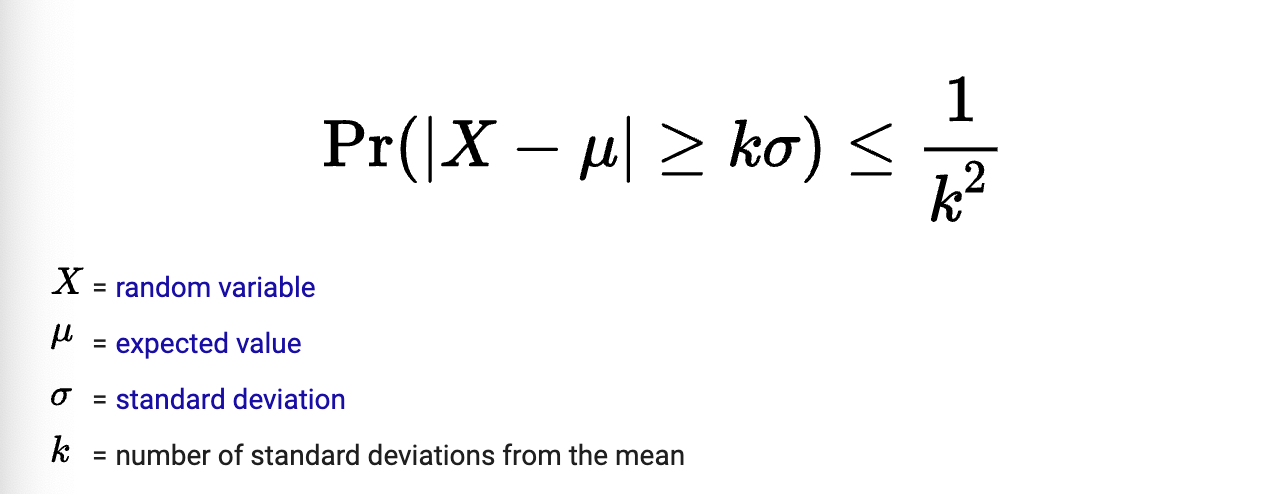
Chebyshev’s Inequality

guarantees only 1/K² values will be found within a specific distance from the mean of a distribution

Z-score

(data point - mean)/standard deviation

Percentile

P(k) = percent of observations less than or equal to k

Quartiles

Q1 = 25% of the data is less than this = 25th percentile

Q2 = 50% of the data is less than this = 50th percentile

Q3 = 75% of the data is less than this = 75th percentile

IQR

middle 50% of observations -> Q3 - Q1

Fences

cutoff values for determining outliers

    Upper fence: Q1 - 1.5(IQR)

    Lower fence: Q3 + 1.5(IQR)

5 Number Summary

min, Q1, M, Q3, max

Boxplot

Number line long enough to include max and min values with vertical lines at Q1, M, and Q3

• Upper and lower fences labeled

• Whiskers: lines from Q1 to smallest value and Q3 to largest value minus the outliers

• Outliers marked with asterisk

• Median is in the middle of box if data is not skewed

Explanatory Linear (positive)

increase in x -> increase in y

Explanatory Linear (negative)

increase in x -> decrease in y

Explanatory Nonlinear

some pattern, but not linear

Explanatory No Relation

almost random

Positive association

increase in x -> increase in y

Negation association

increase in x -> decrease in y

Linear correlation coefficient + rules

measure of strength and direction of the relationship of two variables

1. The linear correlation coefficient is always between –1 and 1, inclusive. That is, –1 ≤ r ≤ 1.

   2.  If r = + 1, then a perfect positive linear relation exists between the two variables.

   3. If r = –1, then a perfect negative linear relation exists between the two variables.

   4. The closer r is to +1, the stronger is the evidence of positive association between the two variables.

   5. The closer r is to –1, the stronger is the evidence of negative association between the two variables.

Line of best fit

a line which is drawn from two points that best express the data

Residual

the difference between the observed value of y and the predicted value of y

Scope of the model

the range of values that the data set applies to based on what makes sense