Digital Signal Processing CGSC433

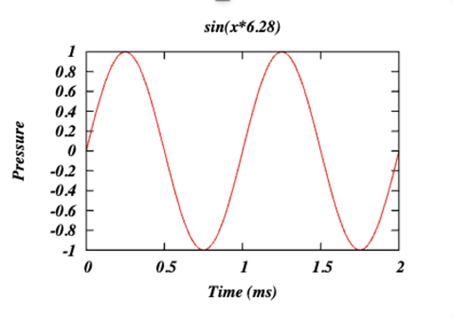
representation of time and amplitude can be

continuous or digital (discrete)

continuous

continuous line with numbers having a theoretically infinite number of decimal places

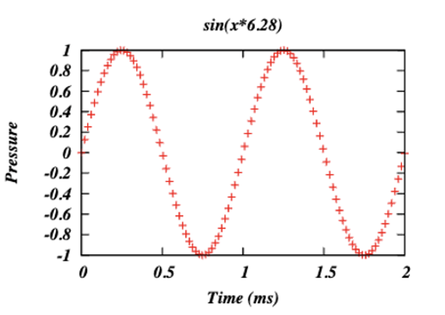
digital (discrete)

sequence of separate points; number of decimal places is always limited- no solid line

digital devices such as computers can

only store a finite amount of information

no computer can store the exact value of pi because

it has infinitely many decimal places. Computers can only store this number to a certain number of decimal places

two important aspects of conversion

how precisely we measure time-sampling and how precisely we measure amplitude-quantization

sampling is

how frequently we take measurements of the signal in time

sampling interval is quoted as

a frequency

sampling rate (in Hz)

is the number of sampling points (intervals) per second

10,000 samples/sec= 10,000 Hz

10 kHz

the higher the sampling rate

the more accurate the digital approximation

not enough sampling points

not going to resemble the original wave

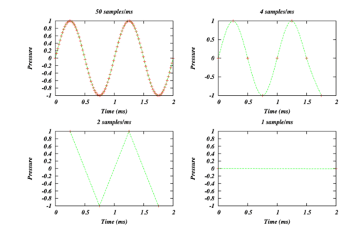
sampling: high resolution

sampling: moderate resolution

sampling: low resolution

analog devices

can store continuous air pressure variations into continuous electrical signals- computers can't do this

examples of analog devices

tape recorders, vinyl records

on computers signals get stored as

digits-they are digital devices

all acoustic signals in computers are

discrete

analog-digital conversion

1. limit the number of places after the decimal point on the time axis=sampling

2. limit the number of places after the decimal point on the amplitude axis=quantization

sampling rate

# of times per second that we measure the continuous wave in producing a discrete representation of signal

the signal must be sampled

often enough so that all important information is captured

to capture a 100 Hz periodic wave you need

at least 2 samples per cycle--> 200 samples per second

nyquist frequency

highest frequency component that can be captured with a given sampling rate

the nyquist frequency is

1/2 the sampling rate

two sampling rates. A. a low sampling rate that distorts the original sound B. a higher sampling rate that closely approximates the original sound wave- 4 cycles

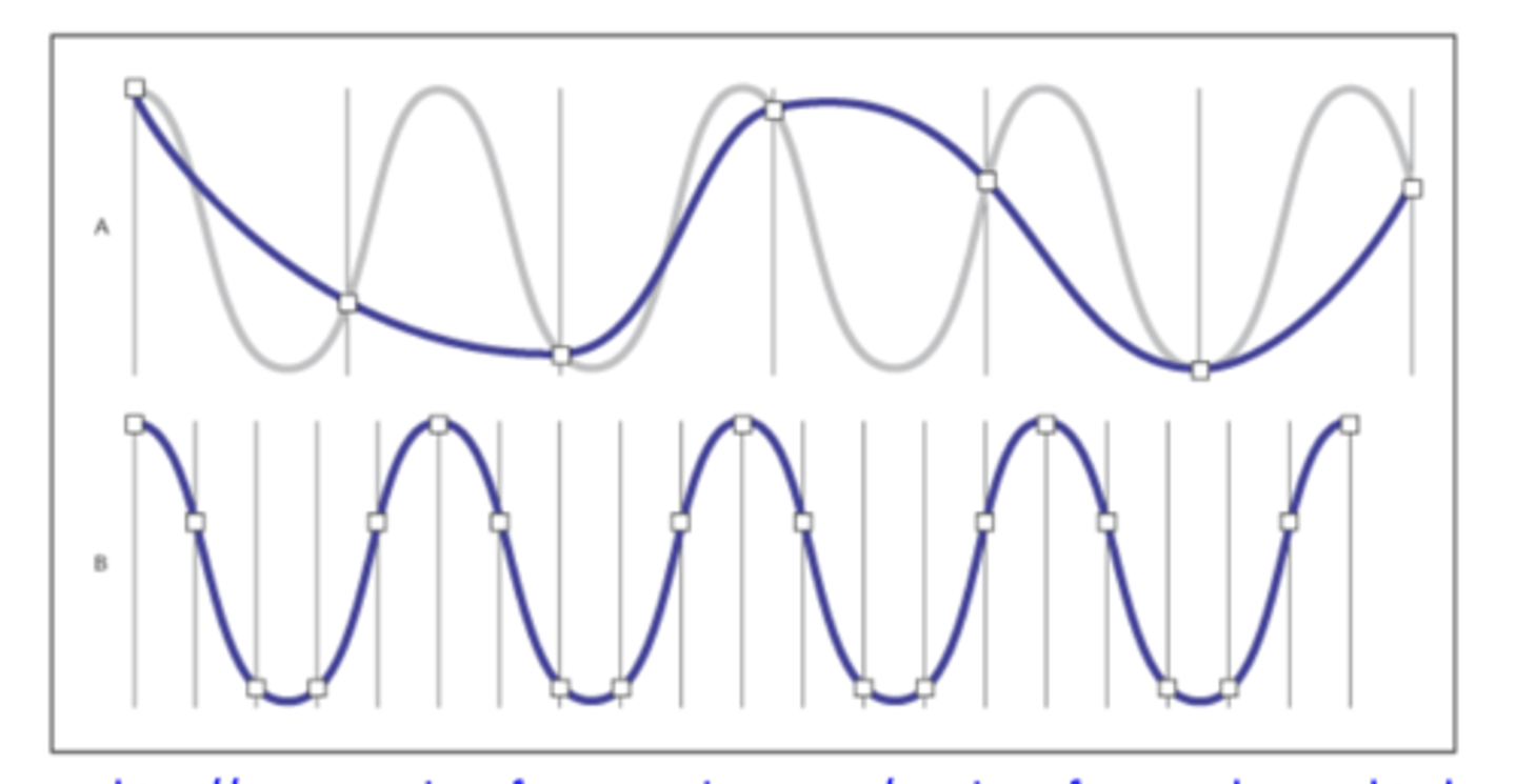
using .5 ms is

very beneficial

if we take samples less frequently

it is not capturing the information well

if continuous signal contains frequency- nyquist frequency

the sampled waveform will have a completely different frequency from that in the original continuous signal-misrepresentation-aliasing

misrepresentation is called

aliasing

to avoid aliasing we can

increase the sampling rate and filter out high frequencies

traditional 20 kHz sampling rate

for speech: any component with a frequency >10kHz will not be captured, BUT it will introduce alias components into the discrete signal

anti-aliasing

it is always necessary to use low-pass filters to block out high frequencies

how to find the cutoff frequency of an anti-aliasing filter

it is half the sampling rate- 16,000Hz/2=8,000 Hz- same thing as nyquist frequency it is HALF

what rate should we sample speech at?

it depends on what we are going to use the recordings for!

the highest frequency that young ears can perceive is

20kHz, so to ensure that all perceptible frequencies are represented, we must sample at 2x20kHZ=40kHz

most of the information relevant to distinguishing speech sounds is

below 10kHz, so high quality speech sound is still obtained at 20kHz sampling rate

for vowels most of the relevant information is below

5kHz, so we can get away with a sampling rate at about 10kHz for analyzing just vowels

energy in fricatives is

higher requiring a sampling rate around 16-20kHz

phones including cell phones have a sampling rate of

8 kHz

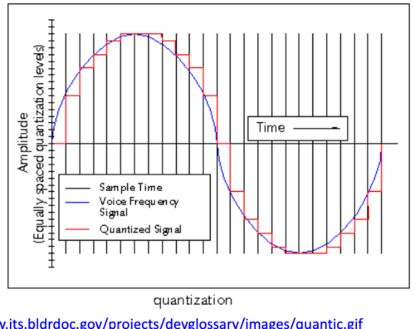
quantization refers to

how finely we chop up the amplitude scale

the continuous amplitude scale is divided into

a finite number of evenly spaced amplitude values

the higher the quantization rate

the more accurate the digital approximation

digital numbers

computer world, limited choices, discrete values

computers handle integers (1,2) better than

decimals (0.01, 0.02 etc.)

acoustic waveforms are stored as

sequences of integers

size of integer

determined by the number of bits (binary digits) used

the larger the number of bits

the greater the amplitude resolution

speech encoding

8, 12, 16 bit quantization

quantization rate is quoted in

bits

a bit can either be

0 or 1

with 1 bit we can only represent

two numbers, 0 or 1

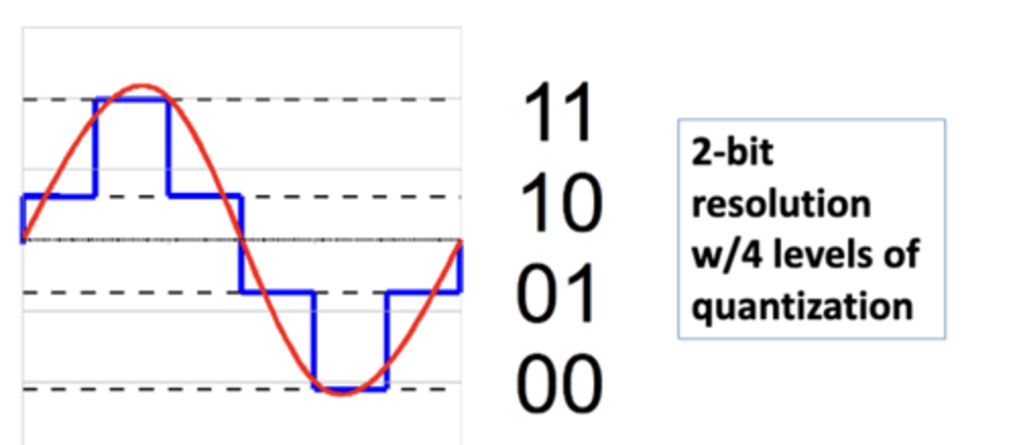
with two bits we have

four possibilities: 00, 01, 10, 11

generally using n bits we can represent

2^n levels of amplitude

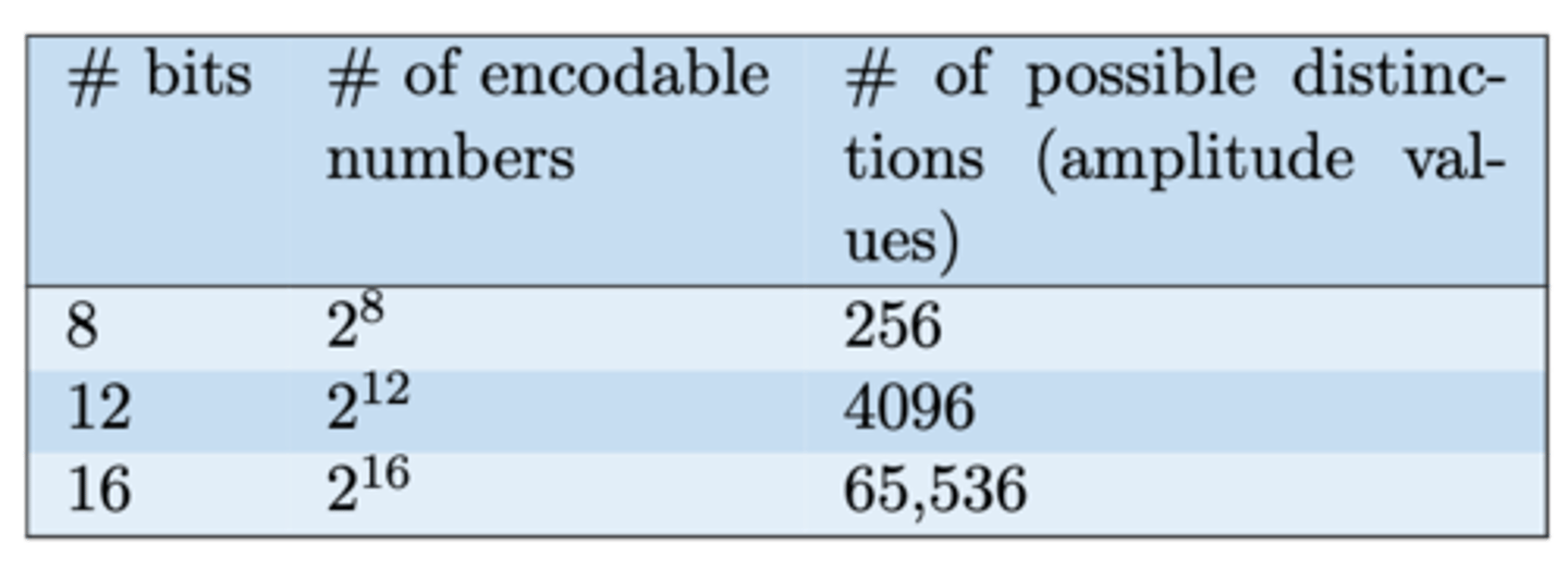
8 bits, 2^8 encodable numbers

256 possible distinctions (amplitude values)

12 bits, 2^12 encodable numbers

4,096 possible distinctions (amplitude values)

16 bits, 2^16 encodable numbers

65,536 possible distinctions (amplitude values)

2 bit resolution with

4 levels of quantization

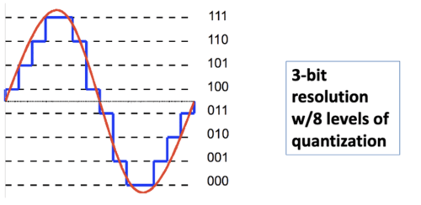
3 bit resolution with

8 levels of quantization

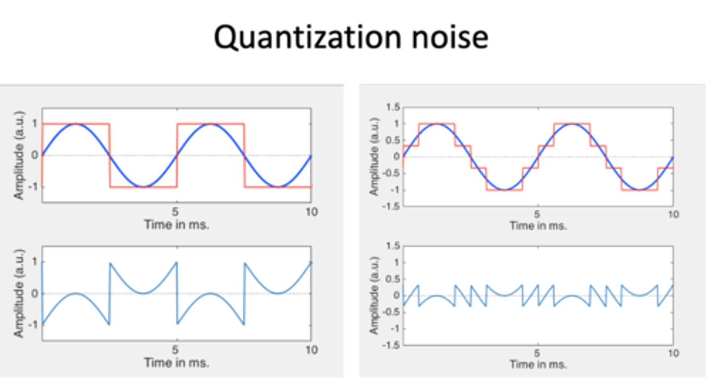
the act of quantization introduces

some error into the signal, which is called quantization noise

quantization noise

error in the signal

quantization noise is

the difference between the actual amplitude of the analog signal and the amplitude of the digital representation

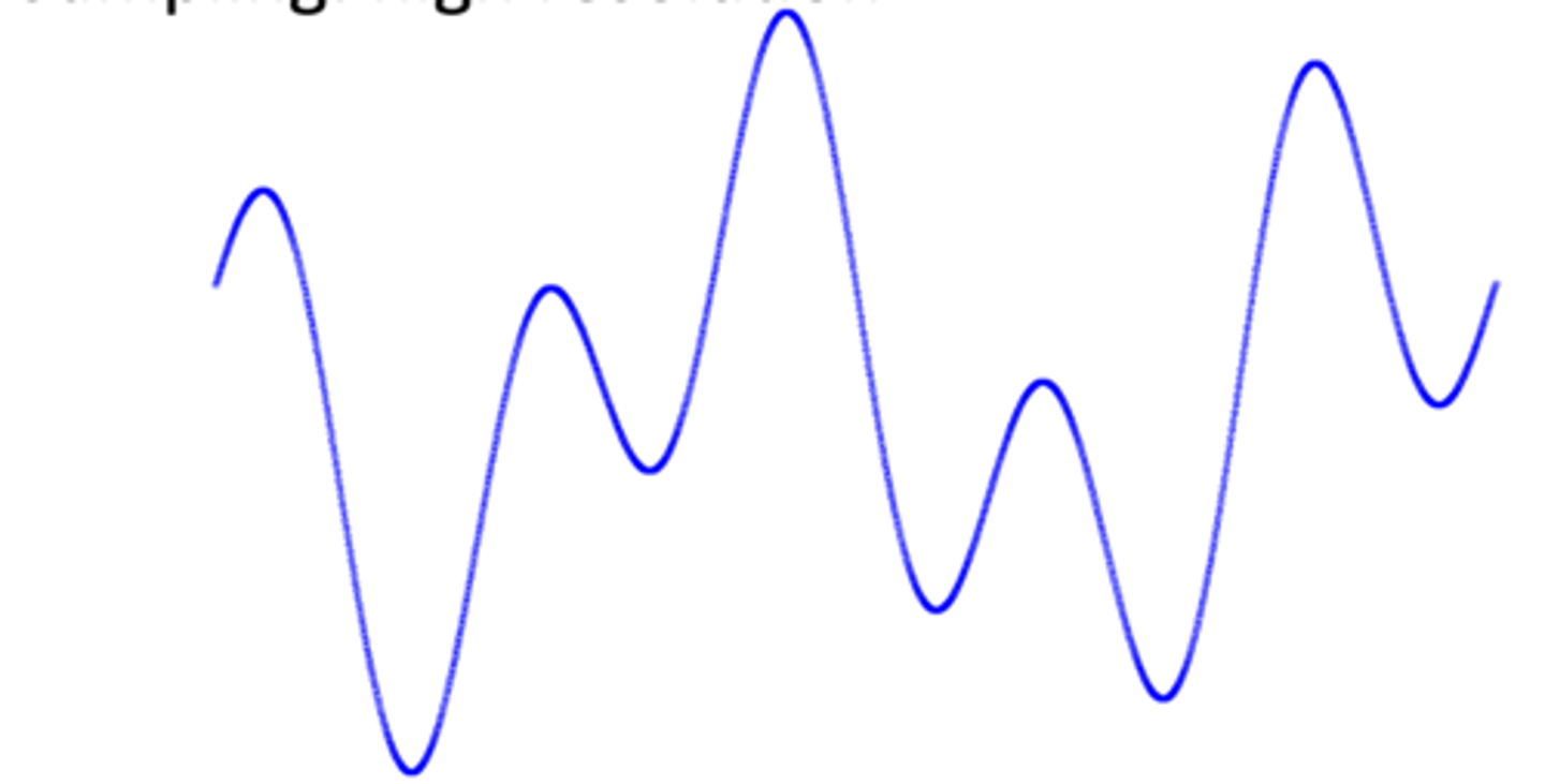
subtract red from blue and get the graph below

too much noise

affects the way the sound is

the relative loudness of quantization noise is called

signal-to-noise ratio

smaller ratios mean

the noise has a bigger effect

larger ratios mean

the noise has a smaller effect

signal-to-noise ratio is typically expressed as

a ratio from number of possible amplitude steps to 1; for 16 bit quantization: 65,536:1

noise has a smaller effect for

65,536:1 than for 4,096:1 (12 bit)

the ratio is the best possible in principle given the

level of quantization

if the amplitudes in the actual signal do not make use of the full range of values

the actual signal-to-noise ratio may be smaller

how many amplitude steps can be represented if we are using 10 bits?

2^10=1024

what is the maximum signal to noise ratio of 1024 amplitude steps/bits?

1024:1 (number of amplitude steps/bits to 1)

when recording

you are supposed to keep the signal amplitude as high as possible- you are supposed to keep the bar in the green zone without going into the red zone

red zone

clipping

keeping within the green zone

keeps the actual signal-to-noise ratio high (so the quantization noise has a smaller effect) because you are using the full amplitude range

techniques for investigating digital signals include

digital filters, autocorrelation, RMS amplitude, Fast Fourier transform, linear predictive coding, and spectrograms

digital filters

removes low or high frequency components from the signal

autocorrelation

tracks pitch changes over time

RMS amplitude

measures acoustic intensity (loudness)

Fast Fourier Transform (FFT)

decomposes complex waves into their single component parts

linear predictive coding

allows examination of broad spectral peaks

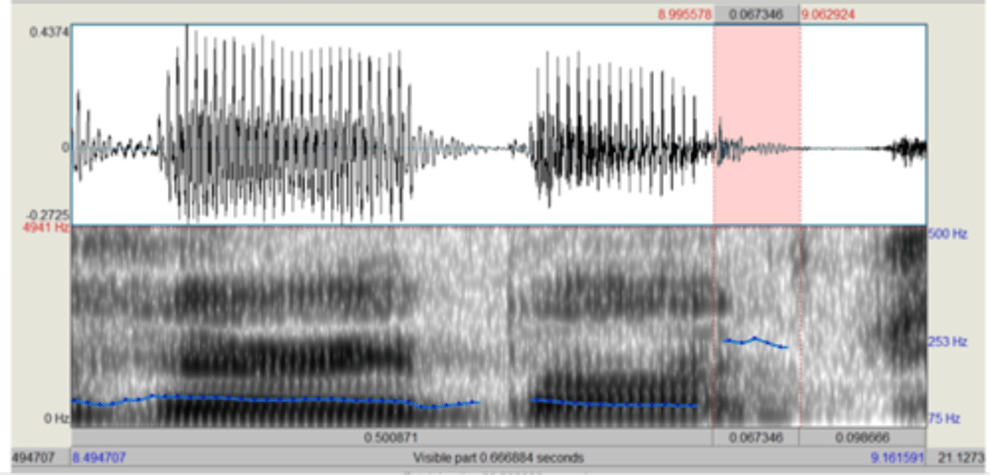
spectrograms

shows spectral changes over time

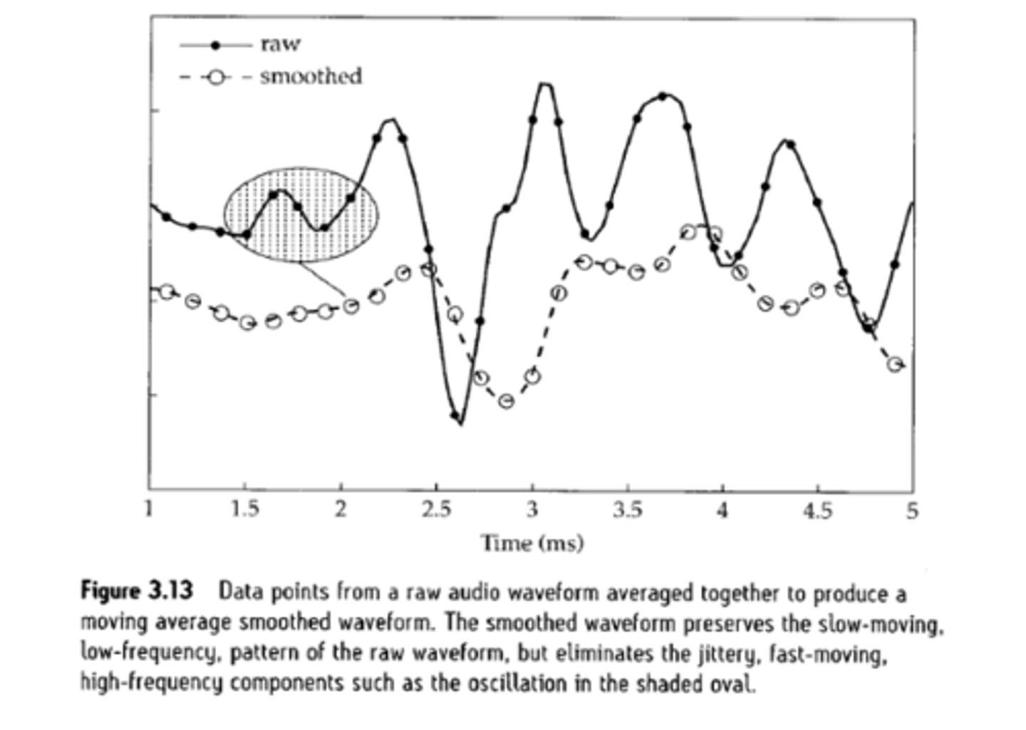
we can construct a low pass filter by calculating the

moving average- this eliminates the high frequency bumps- the signal is transformed to preserve lower frequency components

longer windows will create

smoother signals, but with worse time resolution- not being able to see changes over time very well because they have been smoothed over

when we speak our F0 is always

changing at least slightly

there are many methods to tracking fundamental frequency over time, one of which is

autocorrelation

tracking fundamental frequency- the idea is to pick some interval of the speech signal, make a copy of it and then

1. shift the copy of itself over by 1 sample and see how well the copied interval correlates with the actual wave

2. then shift it by 2 samples and check the correlation

3. then shift it by 3 etc.

4. after some predetermined number of shifting, stop and choose the best correlation

when shifting the interval by 50 and 90 samples

the lag doesn't correlate well with the original

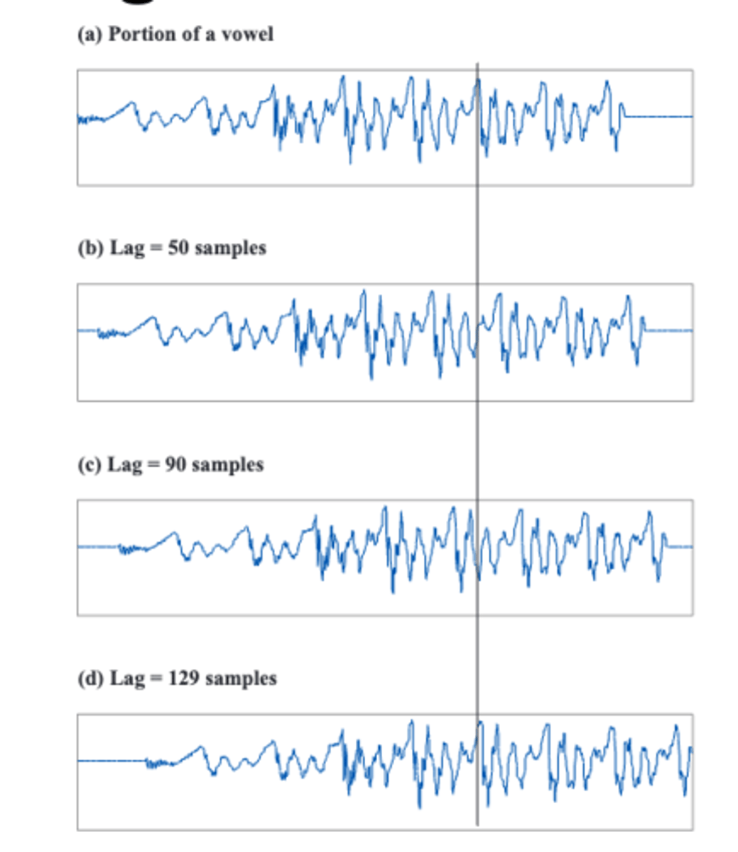
shifting by 129 samples gives

the best correlation, the lag duration is our best guess of the period of the wave

since the sampling was done at 16,000 samples/s (16 kHz) we calculate the F0 by

129/16000 gives us the length of the lag duration in seconds0 the period so its inverse 16000/129 is the frequency=124.031 Hz

in praat the possible frequency range is

75-500 Hz these frequencies determine the minimum and maximum possible lag durations

potential problems with autocorrelation

pitch doubling and pitch halving

pitch doubling

occurs when one cycle of the waveform has two halves that look roughly the same and the autocorrelation method mistakes them as separate cycles

when pitch doubling happens

it tracks the pitch as double the actual value

pitch halving

occurs when alternating pitch periods are more similar than successive periods and the autocorrelation method mistakes two adjacent pitch periods as part of the same cycle

when pitch halving occurs

it tracks the pitch as half the actual value

Root Mean Square (RMS) amplitude is

a measure of the energy in a complex wave

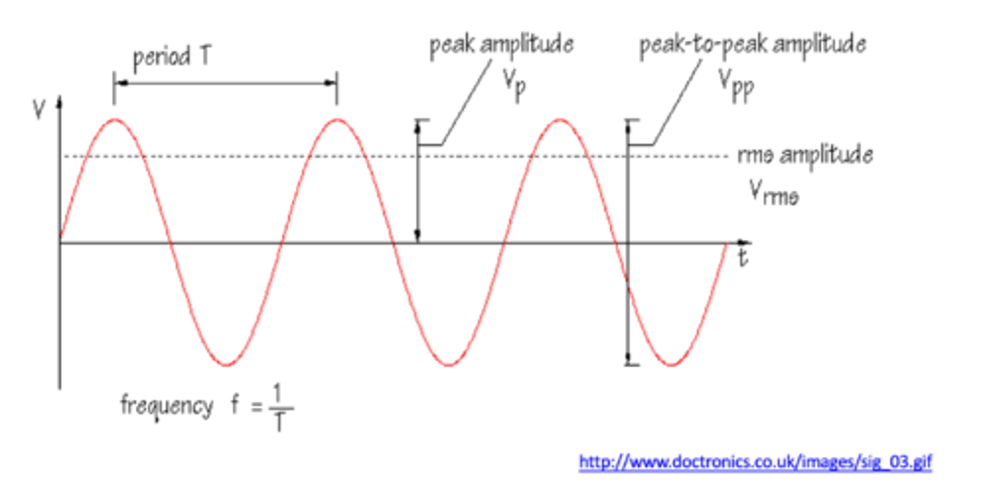
RMS amplitude calculates

the average amplitude over time

RMS amplitude more closely correlates to

perceived loudness than raw amplitude does