C MODEL DIAGNOSTICS & SELECTION

Linear Model

• Y₁, … , Y_n indep

  • Y_i ~ N(μ_i, σ²)

• Constant variance → homoscedasticity

• μ_i = x_iβ

  • Coefficients are linear

GLM

• Y₁, … , Y_n indep

  • Y_i ~ Exponential Family Distr

• Don’t require homoscedasticity

• g(μ_i)= x_iβ

  • Link function

exponential function

GLMs:

• Y_i can be any distr from _____ Family

• A _____ of the mean is linearly related to the predictors instead of mean itself

• Var doesn’t have to be constant

Linear Regression:

• Least Squares & MLE will give same coefficients

  • NOT the case for GLMs!

Systematic

Components of a GLM → _____ Component

• Var explained by lin comb of predictors

• g(μ_i)= x_iβ + offset

Random

Components of a GLM → _____ Component

• Var NOT explained by systematic component

  • Pure random var ε_i

  • Var from variables not included in model

function dispersion

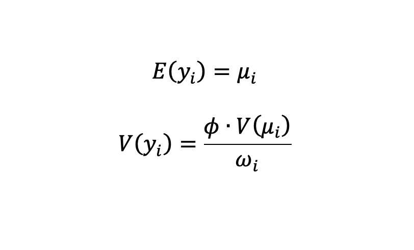
GLM → For observation y_i:

• See pic for mean & var formulas

• V(μ_i) = var of distr as a _____ of mean

• ϕ = _____ parameter

• ω = weight

Link Function

Specifies relationship between random & systematic components of GLM

• Applied to systematic component

• Improves predictive power of model

• Applied to MEAN

link explanatory coefficients fit

Steps to constructing a GLM:

1. Choose distr for response → f(y)

2. Choose _____ function → g(μ)

3. Choose _____ variables x to be modeled → x_i

4. Collect indep obs → y_i

5. Fit model by estimating _____ → β (and ϕ)

6. Evaluate model _____ → residuals

Transformation multiplicative

Applied directly to response var

• Helps make relationship more linear

  • Addresses non-normality

response mean

Transformation vs Link Function → Application

• Transformation → apply directly to _____

• Link → apply to _____

yes no

Transformation vs Link Function → Affects Variance?

• Transformation → _____

• Link → _____

multiplicative distribution

Transformation vs Link Function → Error Component on original scale of y

• Transformation → distorts error

  • May make it _____

  • Change its _____

• Link → does NOT affect error

retains bias interpretability normal linear

Benefits of Link Function

• _____ original data

• Introduce less _____

• Preserve model _____

• Facilitate model comparisons

• Handles non-_____ response variables

• Accounts for non-_____ relationships

Identity Normal

_____ Link → g(μ) = μ

• Domain = (-∞, ∞)

• Canonical: _____

Log Poisson

_____ Link → g(μ) = lnμ

• Frequency/count data

• Domain = (0, ∞)

• Canonical: _____

Power Gamma Inverse Gaussian

_____ Link → g(μ) = μ^p

• Right-skewed data

• Domain = (0, ∞)

• Canonical:

  • _____ → p = -1

    • 1/μ

  • _____ → p = -2

    • 1/μ²

Logit Binomial

_____ Link → g(μ) = ln(μ/(1-μ))

• Probabilities

• Odds = μ/(1-μ)

• Domain = [0,1]

• Canonical: _____

Distributions

Instructions for model on how to generate values

neg skewed patterns

Considerations in choosing distribution:

• Can response be _____?

• Discrete or cts?

• Is data _____

• Noticeable _____

1

Normal Distr → Var(μ) =

• Not impacted by mean

u(1-u)

Binomial Distr → Var(μ) =

u

Poisson Distr → Var(μ) =

u²

Gamma Distr → Var(μ) =

u³

Inverse Gaussian Distr → Var(μ) =

u(1+ku)

Negative Binomial Distr → Var(μ) =

u^p

Tweedie Distr → Var(μ) =

Binomial Logit

_____ Distribution:

• Discrete

  • Captures prob of event occurring

  • Best used for binary response

• Canonical Link → _____

• Var(μ) = μ(1-μ)

Logistic Regression

Binomial distr + Logit link

• Use logistic function to convert log(odds) to a probability

Bernoulli Binomial

_____: prob of success in a single trial

_____: collection of multiple indep Bernoulli trials

Poisson Log

_____ Distribution:

• Discrete

  • Best for count data

  • GLM implementation allows cts data

    • Rates or frequency

• Canonical Link → _____

• Var(μ) = μ

Overdispersion

When data has larger var than predicted by regression

Neg Binomial Quasi Poisson

Poisson has mean = var

Need to adjust for overdispersion if not the case!

• Use another distr

• Use _____ _____

  • ϕ = 1

  • Scale var using ϰ

  • V(y) = μ(1 + ϰμ)

• Use _____-_____

  • Scale var using ϕ

    • V(y)= ϕ μ

  • β coefficients same as Poisson

  • Larger SE

Gamma Inverse Gamma severity power

_____ Distribution:

• Right-skewed, non-neg data

  • Use _____ _____ for extreme right skew

• Commonly used for _____

• Canonical Link → ____

Tweedie power

_____ Distribution:

• Handles data that’s:

  • Clustered around zero

  • Right-skewed

• If 1<p<2 → gives compound Poisson-Gamma

  • Discrete & cts → freq & sev

• Canonical Link → _____

  • g(μ) = μ^1-p

• Var(μ) = μ^p

Poisson Gamma

_____ _____ Compound Distr

• Tweedie where 1<p<2

• Discrete & cts

• No canonical link

• Var(μ) = μ^p

Coefficient SE

Var of coefficient estimate from pop avg

• 95% CI = b ± 2 SE(β)

Statistical Significance true effect

_____ _____: determines if b is far enough from 0 → β=0?

• If observed relationship is likely due to _____ _____ rather than random chance

  • Doesn’t necessarily mean impact on response is big

• Compute z or t-value

  • t* = b/SE(β)

30 pop sd

When to use t-test for statistical significance?

• If n < ____

• _____ _____ unknown

Variable Selection

• Balance efficiency & interpretability

• Too many variables lead to overfitting

context exploratory bivariate analysis

Variable Selection → Qualitative Approach

• Relies on understanding of data & _____

• Findings from _____ phase

  • _____ _____ → correlations

  • Non-linear relationships

Interaction Variables

Variable Selection → _____ _____

• For joint impact on response variables

• Con: hard to interpret

  • Don’t add just bc there’s correlation!

Statistical Significance

Variable Selection → _____ _____

• Generally avoid using variables that aren’t significant

criteria

Forward/Backwards Selection _____

• Typically uses:

  • Adjusted R2

  • AIC

  • Mallow’s Cp

null criteria significance

Forward Selection

• Start w/ _____ model → only intercept

• Explanatory variable examined one at a time

  • Set _____ that allows variables to enter regression

• Add variable w/ best improvement

  • Can’t be removed once added

• Stop when adding another var no longer improves model

• Cons:

  • _____ of existing variable can change as other var are added

    • May end up w/ variable that aren’t statistically sig in model

  • Not flexible

full predictive flexible

Backwards Algorithm / Deletion

• Start w/ _____ model

• Set criteria that allows variable to be removed

  • Can’t be added once removed

• Stop when removing another variable doesn’t improve model

• Pros:

  • Easier to account for when variables have greater _____ power together

  • Preferred over forward selection

• Con: not _____

Order matters

Cons of Forward/Backward Selection

• Not flexible → can’t add/remove variables once removed/added

• _____ _____ when predictors are correlated

  • Not guaranteed to find best model

Step Wise alternate

_____ _____ Selection

• Blend of forward& backwards selection

• Initial model can be null, full or fitted model

• _____ between adding/removing variable steps

• Pro: flexible → ALL variables evaluated at each step

• Con: computational complexity

Marginality

Higher power terms will dominate regression

• x is marginal to x²

• x¹, x² are marginal to interaction x¹x²

Marginality Principle

If you include a higher power / interaction term, you must include all marginal terms

• Removing marginal terms is statistically meaningless

group time periods

ω_i = Weight of observation y_i

• Used when:

  • Observations contain _____ info

  • Adjust for diff _____ _____

scaling variance

Offset: optional constant term to linear predictor

• Acts as _____ factor

• Can vary for each obs

• Affects _____ too!

  • Coz link may make it multiplicative

predetermined deductibles directly exposure

When to add offset term:

• Incorporate _____ values

  • _____

• Response _____ varies based on other measures

  • _____ → policy length, # of claims, mileage

MLE

Estimate parameters s.t. observed sample is most likely

Likelihood

Plausibility of set of parameters given observed sample & model

• Only useful for comparisons

• Not useful by itself

Likelihood Function

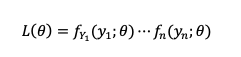
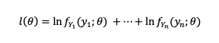
Log Likelihood Function

Find max by taking deriv wrt θ

Residuals

Measures model fit

• Represents portion of var that model doesn’t explain

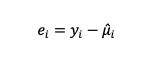
Raw Residuals

Diff between observed vs predicted values

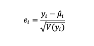
Pearson Residuals

Standardized diff between observed vs predicted values

• Accounts for heteroscedasticity (diff var)

Coefficient of Determination

_____ _____ _____ (R²)

• Prop of var in response that’s explained by model

• Null Model

  • Only intercept → p = 1

  • Lowest R²

• Saturated Model

  • p = n

  • Highest R²

Null Deviance

Compares log likelihood of saturated vs null model

• 2ϕ ( ln L_Sat - ln L_null )

Residual Deviance

Compares log likelihood of saturated vs proposed model

• 2ϕ ( ln L_Sat - ln L_Prop )

• Smaller = better fit

  • df = n-p

  • If (Residual Deviance) / (n-p) > > 1 → poor fit