Chapter 3: Investigating and modelling linear associations (Bivariate Data)

Investigating and modelling linear associations (Bivariate Data).

Linear Regression

Linear regression fits a straight line to bivariate data, allowing predictions. The regression line shows how the response variable changes with the explanatory variable.

The Least Squares Regression method is used to find this line in General Maths.

Residuals and Least Squares Line

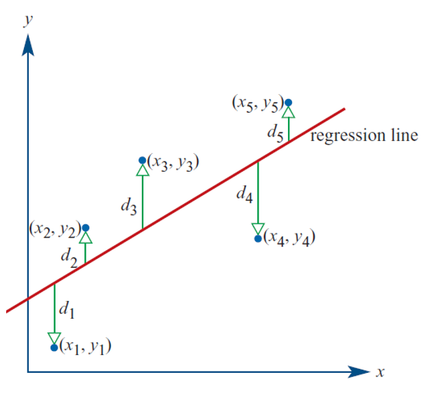
A regression line (not necessarily the least squares line) is drawn to a scatterplot. The vertical distances (𝑑₁, 𝑑₂, 𝑑₃, 𝑑₄, 𝑑₅) between the points and the line are known as residuals. The least squares line minimizes the sum of the squares of the residuals (𝑑₁² + 𝑑₂² + 𝑑₃² + …), balancing data points on either side.

Squaring the residuals prevents the sum from being zero and avoids multiple solutions.

Assumptions made for LSR

Assumptions for the least squares regression:

• The data is numerical.

• The data is linearly related.

• There are no clear outliers.

The least squares line attempts to minimize the gaps (residuals) between the line and the actual points, balancing the data on either side.

Residuals

A residual is the vertical difference (along the y-axis) between the observed data point (scatterplot dot) and the predicted value from the regression line.

• Points below the line have a negative residual value.

• Points above the line have a positive residual value.

Also:

• Data values above the regression line will be above the residual line

• Data values below the regression line will be below the residual line

• Data values on the regression line will be on the residual line

Formula:
- Residual = Actual value – Predicted value

Calculating the least squares regression equation

For the equation y = a + bx:

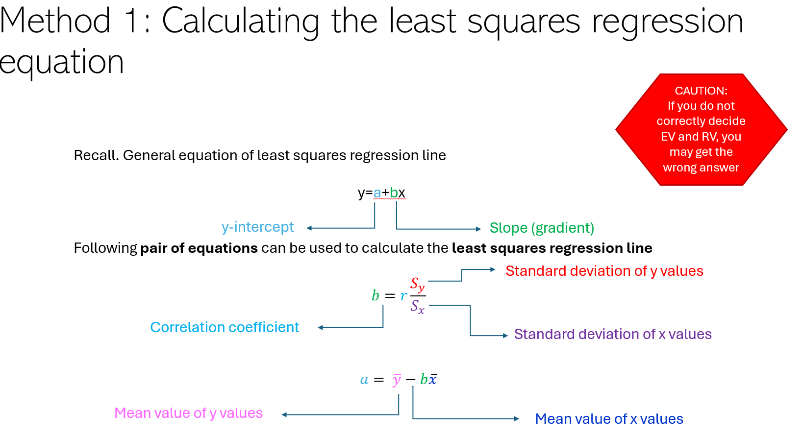
• The slope b is given by: b = (r * sy) / sx

• The intercept a is given by: a = y̅ - b * x̅

For the equation y = c + mx:

• The slope m is given by: m = (r * sy) / sx

• The intercept c is given by: c = y̅ - m * x̅

  Where:

  • y = response variable

  • x = explanatory variable

  • a, c = intercepts

  • b, m = slopes

  • r = correlation coefficient

  • sy = standard deviation of y

  • sx = standard deviation of x

  • y̅ = mean of y

  • x̅ = mean of x

CAS Instructions

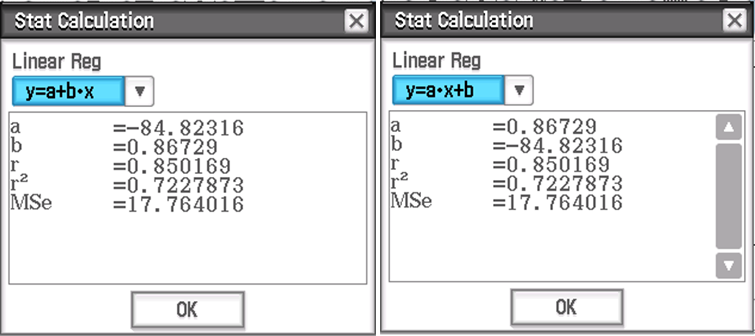
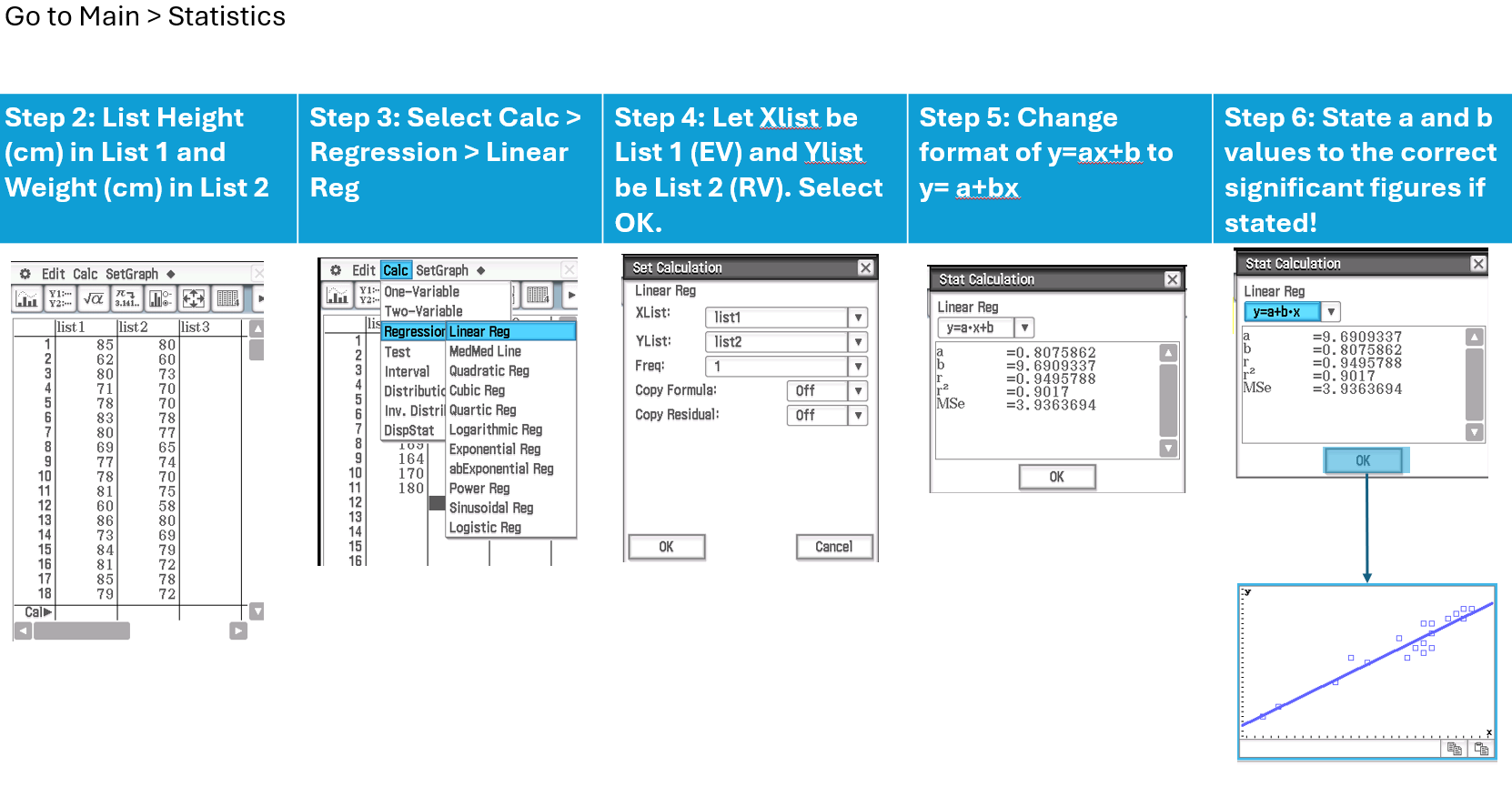
Your calculator can present your residual line either as y = a + bx OR y = ax + b.  Be careful to check!! VCE General maths requires you to use y = a + bx

Interpreting LSR

When using the CAS, the final equation should be written in terms of the worded variables (with units included), not just x and y.

For example, if the CAS gives:

• a = -85 (Note the negative!)

• b = 0.87

The equation should be written as:
Response Variable = Intercept + Slope × Explanatory Variable

Where:

• Response Variable (with units) = -85 + 0.87 × Explanatory Variable (with units).

Selecting Appropriate Points

When choosing points for regression, select values where you can easily determine the x and y values.

For example, if there is a grid, pick a point where the line passes through an intersection of the grid lines, as this will make the calculation simpler and more accurate.

Example of Using LSR

The equation of a regression line that enables the price of a second-hand car to be predicted from its age is:

Price = 35100 – 3940 x age

1. Interpret the slope in terms of the variables price and age.

2. Interpret the intercept in terms of the variables price and age.

3. Use this equation to predict the price of a car that is 5.5 years old.

Interpreting the slope and the intercept of the regression line

For the regression equation y = a + bx:

1. Slope (b):

• If b is positive, y (response variable) increases as x (explanatory variable) increases.

• If b is negative, y decreases as x increases.

• The slope predicts the change in y when x changes by one unit.

2. y-intercept (a):
   The y-intercept predicts the value of y when x = 0.

Interpreting the Slope/Intercept (b/a)

Template for interpreting slope (b):
On average, RV [increases/decreases] by [slope] (units of RV) for each one (unit of EV) increase in EV.

Tips for interpreting the slope:

• Always include the units to justify the context.

• Positive gradient means an increase, negative gradient means a decrease.

Example Interpretation:
On average, apparent temperature increases by 0.9℃ for each one degree increase in actual temperature.

---

Template for interpreting intercept (a):
On average, when the EV is 0 (unit of EV), the predicted RV is (y-intercept) (unit of RV).

Note:

• The intercept may have no meaningful interpretation if x = 0 doesn't make sense in the given context (e.g., a car can't have age 0).

Making Predictions with Linear Regression

Template for Predictions:
Predictions can be made by substituting either a response variable (y) or an explanatory variable (x) into the linear regression equation.

Example:
For the equation:
Ice cream sales ($) = −159.474 + 30.0879 × Temperature (℃)

To predict ice cream sales for a given temperature, substitute the value of temperature (°C) into the equation.

Note: Ensure correct units and significant figures are used when stated!

Interpolation vs Extrapolation

• Interpolation:

  • Predicting within the range of values of the explanatory variable (EV).

  • Reliable, as the prediction is based on observed data.

  • Example: (5.5, 13430).

• Extrapolation:

  • Predicting outside the range of values of the explanatory variable (EV).

  • Unreliable, as it assumes the trend continues beyond the observed data.

  • Examples: (10, -4300), (0, 35100).

Assessing the Least Squares Line Using Residuals

• Calculating the Residual:
  Residual = Raw Data – Predicted Value

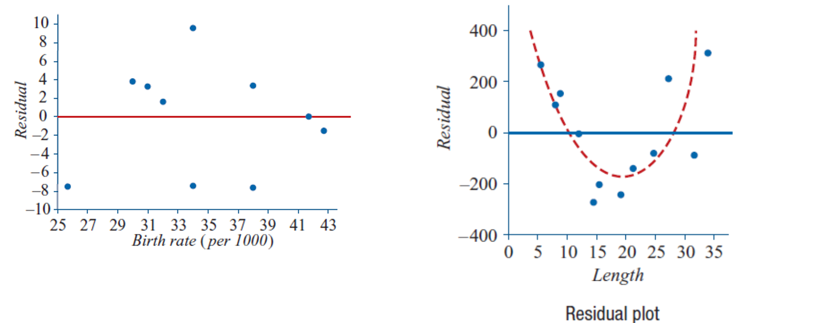
• Residual Plot:
  To assess the suitability of the least squares line, plot all the residuals:

  • Residuals should be randomly scattered above and below the horizontal axis.

  • There should be no clustering of residuals.

  • The distance of residuals from the horizontal axis should be similar across all points.

Positive residual means that the predicted value was too low.

Negative residual means that the predicted value is too high.

Interpreting Residual Plots

• Linear Graph:
  If the graph is linear, there should be no clear pattern in the residual plot. The residuals should be randomly scattered.

• Non-Linear Graph:
  If the graph is non-linear, there will be a clear pattern in the residual plot, indicating that a linear model is not appropriate.

Steps in Regression Analysis (EXTREMELY LONG!)

1. Step 1: Constructing a Scatterplot

   • Observation: No clear outliers, negative linear relationship between life expectancy (RV) and birth rate (EV).

2. Step 2: Calculate Correlation Coefficient (r)

   • Correlation Coefficient (r): -0.8069

   • Conclusion: Strong negative linear relationship.

3. Step 3: Least Squares Regression Line

   • Since r = -0.8069, a linear regression line is appropriate.

4. Step 4: Interpreting the Coefficients (a and b)

   • Slope (b): On average, [RV] increases/decreases by [b, units of RV] for an increase/decrease in [EV] by 1 [unit of EV].

   • Intercept (a): On average, when [EV] is 0, [RV] is [a, units of RV].

5. Step 5: Predictions Using the Regression Line

   • Example: On average, a birth rate of [x] will predict a life expectancy of [calculated RV].

6. Step 6: Using Coefficient of Determination (r²)

   • Interpretation of r²: r²% of the variation in RV can be explained by EV.

7. Step 7: The Residual Plot (Testing Linearity)

   • Residual Definition: Residual = Actual value - Predicted value.

   • Step 7b: Calculating Residuals

     • Calculate residuals by subtracting predicted values from actual values.

   • Step 7c: Constructing a Residual Plot (CAS)

     • Residual Plot Analysis:
       To confirm the linear relationship, use a CAS tool to generate the residual plot. The assumption that there is a linear relationship between RV and EV is confirmed if the residuals are randomly scattered around the zero regression line, showing no clear pattern and no clustering of points.

8. Step 8: Reporting the Results

   • Summary of Findings:
     The relationship between [RV] and [EV] is [strength, direction, form] with a correlation coefficient of r = -0.8069. There are no obvious outliers. The regression equation is:
     [RV, (units)] = a + b × [EV, (units)]

     • The slope predicts that, on average, [RV] changes by [b] (units of RV) for each unit change in [EV].

     • Coefficient of determination (r²): r²% of the variation in RV can be explained by EV.

     • Residual plot: Confirms the appropriateness of the linear model.