Sociology 113: Midterm Review

Nature of Statistics

Stats is the science concerned with studying methods etc. to interpret empirical data

Study of variarion

R studio

R is the engine and R-Studio is the interface

Loading and Processing Data

object-oriented language

functions are verbs and objects are nouns

Language and conventions

Case-sensitive

Functions, Objects, and operators

← is to assign values

* multiplication

== is it true

! is x not equal to y

Using packages

apps on smartphones

Data Structures

Scalar, Vector, Data Frame, Matrix, List

Scalar

numeric, integer, character, or logical cannot hold multiple values of the same or different types

a scalar variable can represent a single number, a single text string, a single logical value (TRUE or FALSE), or a single integer value

Vector

C is combine so it combines a vector aka c(2,9, 9,3)

Can combine twice

V[2] gives second element

V[1:5]

Create logical vectors (one-dimensional array-like structure that contains logical values, which are either TRUE or FALSE)

Data Frame

Excel tables

Takes a lot of vectors and makes a data frame out of it

Access the different type of info using $ sign

You can change the name

Matrix

Table

Matrices has the same info, different from data frame

organize and work with structured data

list

a list is a versatile data structure that can hold elements of different data types such as numeric, character, logical, vectors, matrices, data frames, and even other lists. Lists are similar to vectors, but unlike vectors, the elements of a list can be of different types

Descriptive statistics

statistic is the study of variation and analyzing patterns, that's why is called a variable because it varies

Numerical

Continuous, discrete, ordinal

Continuous

how much would you pay for a slice of pizza (continue for ever)

Discrete

whole number

Ordinal

ordinal data has a clear sequence or hierarchy

education level, economic status, agree strongly agree etc, pain scales

Center

mean (average): modeling that entire variable

Median: the middle

Salaries should use median, not mean because the mean gets skewed with greater values

Spread

range, standard deviation, deviation, variance

Range

max-min (not the best because of outliers)

different from IQR

simple measure of variability and is affected by extreme values in the dataset. However, it does not provide information about the distribution of values within the dataset or the central tendency.

Standard deviation

Divide variance

measure of the dispersion or spread of a dataset. It quantifies the amount of variation or dispersion of a set of values

Variance

how much they deviate from the mean (mean or add up all the values and divide by number of numbers in the dataset)

another measure of the spread or dispersion of a dataset. It is closely related to the standard deviation and provides information about how much the values in a dataset deviate from the mean.

Five number summary

Lowest value, lower quartile, median, upper quartile, highest value

Categorical

binomial/dichotomous, nominal, ordinal

Binomial/Dichotomous

yes or no

Nominal

option best describes race or ethnicity

Ordinal

what the highest level of education

Relative frequencies and proportions

Relative frequency is the proportion of times a particular value occurs in a dataset relative to the total number of observations in the dataset

Proportions are ratios that compare a part to the whole, expressing how much of a dataset belongs to a specific category relative to the total dataset

relative frequencies: relative to the total number

proportions compare a part to the whole

Two-way tables

Two-way tables are useful for analyzing relationships between categorical variables and identifying patterns or associations in the data.

creating multi-way tables

Different types of distributions

Normal, Skewed, Exponential, Uniform

Normal

A normal distribution is like a symmetrical bell, with most data clustered in the middle and fewer data points as you move away from the center. It's smooth, balanced, and described by its mean and standard deviation.

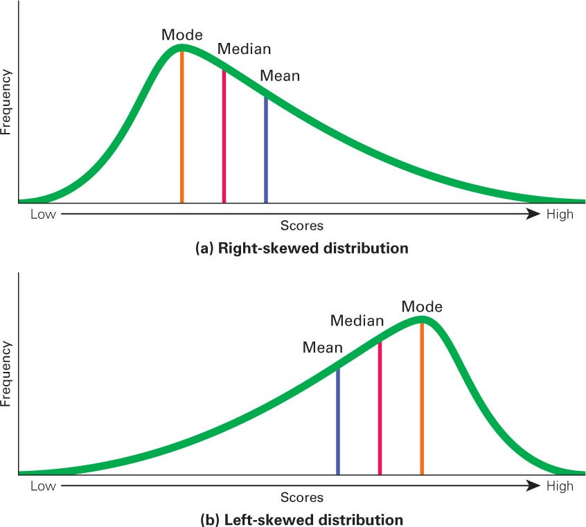
Skewed

Majority of data points cluster towards one side, causing the curve to be asymmetrical

Right Skewed: mode, median, mean

Left Skewed: mean, median, mode

Exponential

Occurrences of events that happen randomly over time, often with a rapid decline in probability as time progresses

Uniform

uniform distribution" refers to a probability distribution where all values within a given range are equally likely to occur

Principles of effective visualizations

need it in .csv, studata.frame(read.csv(“studata.cvs”))

Histogram

a histogram is a graphical representation of the distribution of numerical data. It divides the data into intervals called "bins" and counts the number of observations that fall into each bin. The height of each bar in the histogram represents the frequency or relative frequency of observations in that bin.

Histogram (hist())

Code: hist(yrsincoll) variable inside

Picks axis that seems best but you can change them

Tells you how many times something pops up in the data

Breaking down the code: Hist (yrsincoll, main = “Number of years my closest friends have spent in college”, xlab = "Number of years in college", ylab = "Number of friends", xlim = c(0,5), col = "pink")

Main: Main title xlab:x label ylab: y label xlim: limits of x-axis col: color—must be in ““

Histogram ggplots

Create a data frame from the variable

ggplot(data = testdata, aes(x = yrsincoll))+geom_histogram()

Data frame and type of variable you want to view then the type of graph at the end “+” adds layers and

Add layers to object saved

Box plots

a box plot (also known as a box-and-whisker plot) is a graphical summary of the distribution of numerical data through five key summary statistics: the minimum, lower quartile (Q1), median (Q2), upper quartile (Q3), and maximum.

Median and tells us how data is spread out

5 number summary

Box Plots code

Code: myboxplot <- ggplot(data = studata, aes(x = sleephrs)) + geom_boxplot()

Add the layer of boxplot, you can add a layer of boxplot ontop of a histogram

Pie Charts

Pie charts are useful for visualizing the relative sizes of different categories or proportions within a data set.

Not always as useful

Basic r == pie ()

Ploty and dplyr packages must be uploaded

Bar charts

In R Studio, a bar chart is a graphical representation of categorical data that uses rectangular bars to represent the frequencies or proportions of different categories

ggplot2: Geom_bar

Scatter plots

Scatter plots are useful for visualizing the relationship between two numerical variables, identifying patterns, trends, and outliers in the data, and assessing the strength and direction of the relationship between the variables

Normal distributions and the central limit theorem (Gaussian)

Bell curve shaped, pattern happens all the time

Influenced by a tiny little factors

with a large sample size, the distribution of sample means will be approximately normal, regardless of the original distribution's shape

the mean (μ), which represents the central tendency, and the standard deviation (σ), which represents the spread or variability of the distribution

Identifying outliers

Outside of main distribution

Outliers are data points that significantly differ from the majority of the other data points in a dataset.

warrant special attention in statistical analysis and interpretation.

Interquartile range (IQR)

different from range

Q3-Q1 (half of the values)

Outliers: 1.5*IQR below and 1.5*IQR above

Code: lower_bound <- Q1 - 1.5 IQR & upper_bound <- Q3 + 1.5 IQR

outliers <- happyworld[(happyworld$Cantrilscore > upper_bound | happyworld$Cantrilscore < lower_bound), ]

Q1 <- quantile(happyday$happiness, 0.25) and Q3 <- quantile(happyday$happiness, 0.75)

Z-scores

how many standard deviations a data point is away from the mean of a dataset. It indicates how far a data point is from the mean, in terms of standard deviation units

To figure out how many standard deviations something is from the value, we subtract it by the mean and divide by standard deviation (then it must be below 3 and -3 if not it is an outlier )(e.g., ±3)

z= x-mean/ sd

identifying outliers, comparing data points from different datasets, and standardizing data for statistical analysis

68-95-99.7 rule

empirical rule; statistical guideline that describes the approximate percentage of data within certain standard deviations from the mean in a normal distribution

68.27% of data points fall within 1 SD above or below the mean

95.45% of data points fall within 2 SDs above or below the mean

99.73% of data points fall within 3 SDs above or below the mean

• Only 0.3% of all data are 3D way from the mean

Standardizing variables

technique used to rescale variables to have a mean of 0 and a standard deviation of 1

Converting a variable to a z score

scale() converts everything into a z-score

Will calculate the IQR but with z scores to see the outliers

sum(happyday$stdhappiness > 3 | happyday$stdhappiness < -3)

Range of acceptable values

refers to the acceptable boundaries or limits within which a variable or measurement is considered valid

(Z*SD) + Mean = X

Multiply by 3 and -3 to get upper and lower limits

Percentiles

Percentiles are often used to understand the distribution of data and identify specific values that are typical or extreme within a dataset

Pnorm (z) tell you the percentage of numbers higher or lower

it returns the probability that a standard normal random variable is less than or equal to z

Conceptual significance of outliers (and how to handle them)

Get rid of errors while preserving natural variation

Skewness

Skewness is if it is of to the side and it is calculated usign skewness() 

Negatively skewed (left) : mean is higher 

Normal = 0 

Positive skewed (right)= mode peaks first

Kurtosis

the tails needs to be between 2 and -2, this is calculated using the library moments ans code kurtotis ()

indicates whether the distribution is more peaked and has heavier tails than a normal distribution (positive kurtosis), less peaked and has lighter tails than a normal distribution (negative kurtosis), or has similar peakedness and tail behavior as a normal distribution (kurtosis close to zero).

Skewness and kurtosis

skewness describes the symmetry of the distribution, while kurtosis describes the shape of the distribution's tails.

Sampling and the central limit theorem

No matter the kind of variable or sample you always get a normal distribution (therefore you can make predictions from sampling)

Flipping a coin

Seed is random 

Population vs Sample

CLT helps us make assumptions from a population just from one sample

Population: N μ(mean) σ(standard deviation)

Sample: n x(mean) and d(standard deviation)

Degrees of freedom

For sample, the formula is n-1 

Lose a degree of freedom for every parameter that you estimate 

If you do not subtract, then you underestimate the values

number of values in the final calculation of a statistic that are free to vary. It's a concept that's used in various statistical tests and calculations

Z-score

How far a data point is from the mean 

Z-test  (comparing sample to population)

Where sample fits relative to the population

“Teaching demos”

Apply to sample to check is sample is different from population

z.test(sample_mean, mu = 4, SD = 1.5)

Divided by square root of n

~By comparing the calculated z-value to the critical values from the standard normal distribution, you can determine whether to reject the null hypothesis

Standard error

√n

How spread out, but this is about the precision of sampling to the entire population

Average of sample should be about average of population

How confidence you can be about assumptions

Error means uncertain and number are different from expected, variability that isn't being captures

measure of the variability or uncertainty in an estimate, particularly in the context of statistical inference. It quantifies the precision of an estimate by indicating how much it might vary from the true population parameter on average

T-test

see if values from one sample vary from a different sample (equation similar to Z test, but it doesn't rely on normal distribution but a t distribution)

One sample T-test (comparing sample to population)

Tails are bigger, more conservative approach to hypothesis testing

t.test(studata$approx_drinks, mu = 6.5)

How much different, t=11 t value must be less than 0.5 to be confident that it is different

commonly used when you have collected a sample and want to assess whether it is representative of the population from which it was drawn

Two sample T-test

Comparing, two groups of people and could be different sizes (means ) 

Have to be independent, small sample size (<30 ppl) normally distributed or 

More people the more confident we can be 

compare the means of two groups to assess whether there is evidence of a difference between them

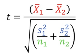
T-statistic 

Subtract means and add together standard errors, variance we could account for, gives sense of confidence that two samples are statistically significant 

hypothesis testing to assess whether the observed difference between the sample mean and the population mean is statistically significan

Unpaired T-test

statistical test used to compare the means of two independent groups to determine if they are significantly different from each other,

The null hypothesis (𝐻0) for an unpaired t-test typically states that there is no difference between the means of the two groups. The alternative hypothesis (𝐻𝑎) suggests that there is a significant difference between the two means.

Paired

Every person in the first sample is PAIRED with someone in the next

a statistical test used to compare the means of two related groups to determine if they are significantly different from each other. It's commonly used when you have paired or matched observations and want to assess whether there is evidence of a difference in their means.

T-distribution

Small sample sizes

a probability distribution that arises in hypothesis testing when the population standard deviation is unknown and must be estimated from the sample data.

Effect sizes~difference between means

Larger sample sizes the smaller differences, shape of distribution –more confidence with low variability 

The study must have enough power to detect effect, if it does not vary as much, how far the mean are and how spread out 

More power detects smaller differences between sample means and be more confident in our results.

• Small effect size: d = 0.2

• Medium effect size: d = 0.5

• Large effect size: d = 0.8

How it is relevant to how spread out

Conceptual foundation of test statistics

Framework of hypothesis testing, a fundamental concept in statistics used to make inferences about population parameters based on sample data.

Null Hypothesis, Alternative Hypothesis, t-statisitc, Sampling distribution under the null hypothesis,

Null Hypothesis

Default assumption about the population parameter(s)

no effect, no difference, or no association between variables.

Alternative hypothesis

It asserts what you hypothesize to be true about the population parameter(s) being tested. It can be one-sided (e.g., greater than, less than) or two-sided (e.g., not equal to)

Test statistic

numerical summary of sample data that measures the degree of compatibility between the observed data and the null hypothesis. It quantifies how far the observed data deviates from what would be expected under the null hypothesis

Sampling distribution under the null hypothesis

Represents the distribution of test statistic values that would be obtained if the null hypothesis were true and helps assess the probability of observing the data given the null hypothesis

p-value

threshold used to determine the strength of evidence against the null hypothesis

The decision to reject or fail to reject the null hypothesis is based on whether the observed test statistic falls beyond the critical value or whether the p-value is smaller than a predefined significance level (e.g., 0.05).

Experimental Considerations

careful consideration of these experimental factors is essential for producing reliable, valid, and ethical research findings that contribute to the advancement of knowledge in the field.

ANOVAs Vs the F-test

ANOVA is a technique used to compare means across multiple groups, while the F-test is a statistical test used to assess the overall significance of the ANOVA model by comparing variances,

the F-test is an integral part of ANOVA and helps determine whether the observed differences between group means are statistically significant

Anovas

ANOVA (Analysis of Variance)

compare the means of three or more groups to determine if there are statistically significant differences between them

Any number of groups, and it will tell you if it has a different mean from the others, not helpful because it doesn't tell you which mean is greater

F-test

F test checks if the variance within the groups/ distribution of each group is smaller across groups

If smth is happening then check with post op test

If the F-test is statistically significant, it suggests that there are significant differences between the group means, and further investigation (e.g., post hoc tests) may be warranted.

Descriptive stats = mean,sd

Descriptive statistics are numerical summaries or measures that provide insights into the central tendency, variability, and distribution of a dataset.

Inference: conclusion of broader population based on sample

Hypothesis testing

Null and alternative hypotheses

H0 or Null= stays the same 

HA or alternative = something happens 

• Keep null hypothesis if you do not have enough evidence to reject it (p >0.5)