MTH 267 - Differential Equations Exam 2 Topics

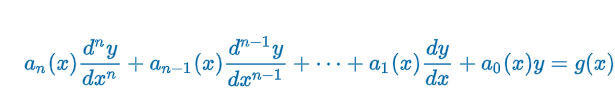
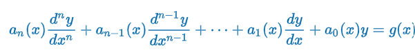
n^th-Order Initial-Value Problem (IVP)

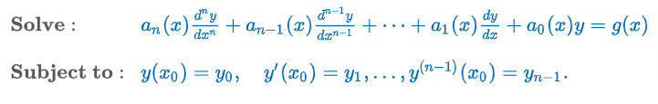
Existence of a Unique Solution Theorem

“Let a_n(x), a_n-1(x), …, a₁(x), a₀(x) and g(x) be continuous on an interval I and let for every x in this interval. If is any point in this interval, then a solution of the initial-value problem exists on the interval and is unique.”

Boundary-Value Problem (BVP)

“linear differential equation of order two or greater in which the dependent variable y or its derivatives are specified at different points”

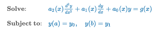
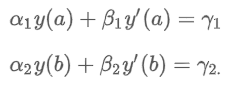
Boundary Conditions (BC)

The prescribed y(a) = y₀ values and a y(b) = y₁

Homogeneous Equations

Equivalently, L(y) = 0

Note: y = 0 is always a solution of a homogeneous linear equation

Nonhomogeneous Equations

Equivalently, L(y) = g(y)

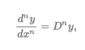
Differential Operator

transforms a differentiable function into another function

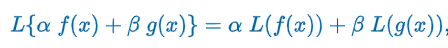
Linearity Property

“L operating on a linear combination of two differentiable functions is the same as the linear combination of L operating on the individual functions”

Superposition Principle

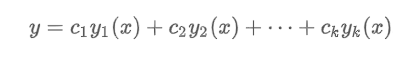
“Let y₁, y₂, …, y_k be solutions of the homogeneous n^th-order differential equation on an interval I. Then the linear combination y = c₁y₁(x) + c₂y₂(x) + … + c_ky_k(x) where the c_i = 1,2,…, k are arbitrary constants, is also a solution on the interval.”

Superposition Corollaries - Homogeneous Equations

(A) A constant multiple y = c₁y₁ of a solution y₁(x) of a homogeneous linear differential equation is also a solution.

(B) A homogeneous linear differential equation always possesses the trivial solution y = 0.

Linear Dependence/Independence

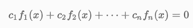
“A set of functions f₁(x), f₂(x), …, f_n(x) is said to be linearly dependent on an interval I if there exist constants c₁, c₂, …, c_n not all zero, such that c₁f₁(x) + c₂f₂(x) + … + c_nf_n(x) = 0

for every x in the interval. If the set of functions is not linearly dependent on the interval, it is said to be linearly independent.”

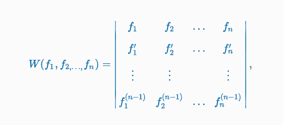
Wronskian

“Suppose each of the functions f₁(x), f₂(x), …, f_n(x) possesses at least n - 1 derivatives. The determinant (Image) where the primes denote derivatives.

Criterion for Linearly Independent Solutions

Let y₁, y₂, …, y_n be n solutions of the homogeneous linear -order differential equation on an interval I. Then the set of solutions is linearly independent on I if and only if W(y₁, y₂, …, y_n) ≠ 0 for every x in the interval.”

Fundamental Set of Solutions

“Any set y₁, y₂, …, y_n of n linearly independent solutions of the homogeneous linear n^th-order differential equation on an interval I is said to be a fundamental set of solutions on the interval.”

Existence of a Fundamental Set

“There exists a fundamental set of solutions for the homogeneous linear -order differential equation on an interval I.”

General Solution - Homogeneous

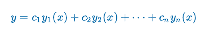
Let y₁, y₂, …, y_n be a fundamental set of solutions of the homogeneous linear -order differential equation on an interval I. Then the general solution of the equation on the interval is y = c₁y₁(x) + c₂y₂(x) + … + c_ny_n(x) where c_i, i = 1, 2, …, n are arbitrary constants.”

Particular Solution

Any function y_p free of arbitrary parameters

General Solution - Nonhomogeneous Equations

“Let y_p be any particular solution of the nonhomogeneous linear n^th-order differential equation on an interval I, and let y₁, y₂, …, y_n be a fundamental set of solutions of the associated homogeneous differential equation on I. Then the general solution of the equation on the interval is y = c₁y₁(x) + c₂y₂(x) + … + c_ny_n(x) + y_p(x) where the c_i, i = 1, 2, …, n are arbitrary constants.”

y = complementary function + any particular solution

y = y_c + y_p

Complementary Function

y =c₁y₁(x) + c₂y₂(x) + … + c_ny_n(x)

General Solution - Nonhomogeneous

Superposition Principle - Nonhomogeneous

Let y_p1, y_p2, …, y_pk be k particular solutions of the nonhomogeneous linear nth-order differential equation (7) on an interval I corresponding, in turn, to k distinct functions g₁, g₂, …, g_k. That is, suppose y_p denotes a particular solution of the corresponding differential equation

a_n(x)yⁿ + a_{n - 1}(x)y^{n - 1} + … + a₁(x)y’ + a₀(x)y = g_i(x)

where i = 1, 2, …, k. Then

y_p(x) = y_p1(x) + y_p2(x) + … + y_pk(x)

is a particular solution of

a_n(x)yⁿ + a_{n - 1}(x)y^{n - 1} + … + a₁(x)y’ + a₀(x)y = g₁(x) + g₂(x) + … + g_k(x)

Reduction of Order

If y₁ and y₂ are linearly independent, then their quotient y₂ ∕ y₁ is nonconstant on I—that is, y₂(x) ∕ y₁(x) = u(x) or ​y₂(x) = u(x)y₁(x).

General Case:

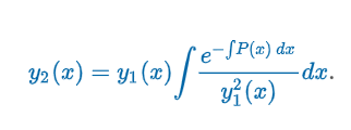
“Let y₁(x) be a solution of the homogeneous differential equation y″ + P(x)y′ + Q(x)y = 0 on an interval I and that y₁(x) ≠ 0 for all x in I. Then (Image) is a second solution.

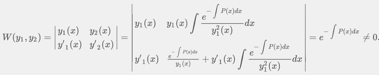
Wronskian w/ Reduction of Order

If is the y₂ solution in the Reduction of Order Formula, then the functions y₁(x) and y₂(x) are linearly independent on any interval I on which is not zero.

m: solution or root of the 1^st degree polynomial equation am + b = 0 (Homogeneous Linear Equations with Constant Coefficients)

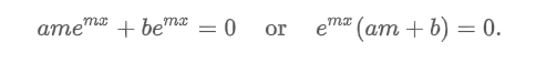
If we substitute y = e^mx & y’ = me^mx into ay’+ by = 0, we get

ame^mx + be^mx = 0 or e^mx(am + b) = 0

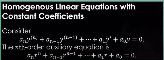
Auxiliary Equation (Homogeneous Linear Equations with Constant Coefficients)

Homogeneous 2^nd-order DE : ay” + by’ + cy = 0 where a, b, & c are constants

Subsitute y = e^mx, y’ = me^mx, y” = m²e^mx

New Equation: am²e^mx + bme^mx + ce^mx = 0 or e^mx (am² + bm + c) = 0

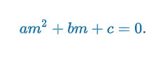
m : root of the quadratic equation

Auxiliary Equation: am² + bm + c = 0

• m₁ & m₂ real & distinct (b² - 4ac > 0),

• m₁ & m₂ real & equal (b² - 4ac = 0), &

• m₁ & m₂ conjugate complex numbers (b² - 4ac < 0)

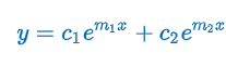
Case 1: Distinct Real Roots (Homogeneous Linear Equations with Constant Coefficients)

Criteria: m₁ & m₂ real & distinct (b² - 4ac > 0)

am² + bm + c = 0 has 2 real unequal roots m₁ & m₂ → linearly independent y₁ = e^m₁x & y₂ = e^m₂x

m₁ = (-b + √(b² - 4ac)) / 2a) & m₂ = (-b + √(b² - 4ac)) / 2a)

y = c₁e^m₁x + c₂e^m₂x

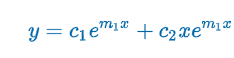
Case 2: Repeated Real Roots (Homogeneous Linear Equations with Constant Coefficients)

Criteria: m₁ & m₂ real & equal (b² - 4ac = 0)

m₁ = m₂ → y₁ = e^m₁x & b² - 4ac = 0 → m₁ = -b/2a

Proof: y₂ = e^m₁x∫(e^2m₁x/e^2m₁x)dx = e^m₁x∫dx = xe^m₁x

m₁ = (-b + √(b² - 4ac)) / 2a) & m₂ = (-b + √(b² - 4ac)) / 2a)

m₁ = m₂ = -b/2a

y = c₁e^m₁x + c₂e^m₁x

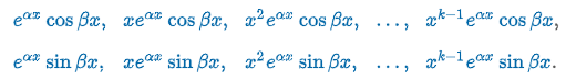
Case 3: Conjugate Complex Roots (Homogeneous Linear Equations with Constant Coefficients)

Criteria: m₁ & m₂ conjugate complex numbers (b² - 4ac < 0)

m₁ & m₂ are complex → m₁ = α + iβ & m₂ = α - iβ were α & β > 0 are real & i² = -1

m₁ = (-b + √(b² - 4ac)) / 2a) & m₂ = (-b + √(b² - 4ac)) / 2a)

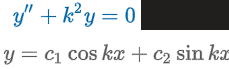
Equation 1 Worth Knowing (Homogeneous Linear Equations with Constant Coefficients)

k: real

DE: y” + k²y = 0

Auxiliary Equation: m² + k² = 0

Roots: m₁ = ki & m₂ = -ki

Solution: y = c₁coskx + c₂sinkx

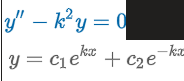
Equation 2 Worth Knowing (Homogeneous Linear Equations with Constant Coefficients)

k: real

DE: y” - k²y = 0

Auxiliary Equation: m² - k² = 0

Roots: m₁ = k & m₂ = -k

Solution: y = c₁e^kx+ c₂e^-kx

Special Case: c₁ = c₂ = ½ → y = 1/2(e^kx + e^-kx) = coshkx

Special Case: c₁ = ½ & c₂ = -½ → y = 1/2(e^kx - e^-kx) = sinhkx

Alternative form: y = c₁coshkx + c₂sinhkx

Higher-Order Equations (Homogeneous Linear Equations with Constant Coefficients)

Repeated Complex Roots (Homogeneous Linear Equations with Constant Coefficients)

m₁ = α + iβ, β > 0 is a complex root of multiplicity k of an auxiliary equation w/ real coefficients, then its conjugate m₂ = α + iβ, β > 0 is also a complex root of multiplicity k

Rational Roots (Homogeneous Linear Equations with Constant Coefficients)

We know that if m₁ = p ∕ q is a rational root (expressed in lowest terms) of a polynomial equation​ a_nmⁿ + … +a_nm +a₀ = 0 with integer coefficients, then the integer p is a factor of the constant term a₀ and the integer q is a factor of the leading coefficient a_n.​

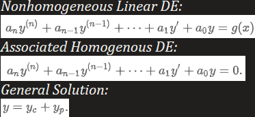
Nonhomogeneous General Solution

General Solution: y = y_c + y_p

y_c : complementary function; general solution of the associated homogeneous DE

y_p :any particular solution of the nonhomogeneous equation

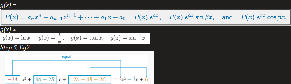
Method of Undetermined Coefficients

Limited to linear DEs such as nonhomogeneous linear DE where

• the coefficients a_i, i = 0, 1, …, n are constants &

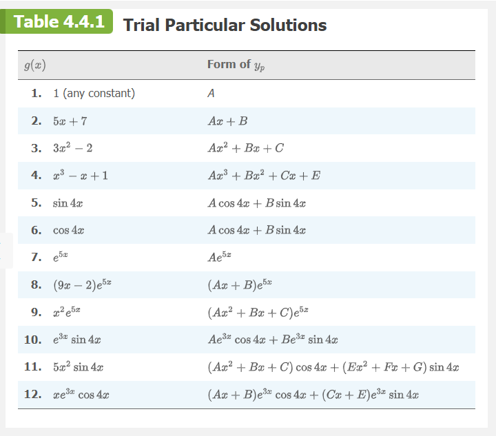
• g(x) is a constant k, a polynomial function, an exponential function e^αx, a sine or cosine function sinβx or cosβx, or finite sums and products of these functions. (Refer to image to what this means)

Steps:

1) Find y_h

• Characteristic Equation

• Identify type of Homogeneous Linear Equations with Constant Coefficient

2) Choose a general y_p

• Look at RHS, the equation will include RHS & it’s derivatives

• Refer to Trial Particular Solutions Flashcard

• Eg. RHS = 3x² → Ax² + Bx + C = 0

3) Derive the general y_p

4) Plug the derivatives into the DE

5) Match elements in LHS w/ elements in RHS

• Eg1. LHS = 2A - 4Ax² - 4Bx + 4C; RHS = 3x² + 0x +1 → 2A + 4C = 0, -4B = 0, -4A = 3

• Eg2. Refer to Image

• Solve

6) Plug into y_p

7) Write y = y_h + y_p

8) Check by plugging solution into DE

Superposition Principle for Nonhomogeneous Equations

y_p = y_p1 + y_p2 +…+ y_pn

(Apply this theorem when g(x) is a combination of allowable functions)

Case 1

No function in the assumed particular solution is a solution of the associated homogeneous differential equation.

The form of y_p is a linear combination of all linearly independent functions that are generated by repeated differentiations of g(x).

Case 2:

A function in the assumed particular solution is also a solution of the associated homogeneous differential equation.

Linear 1^st-Order Revisited

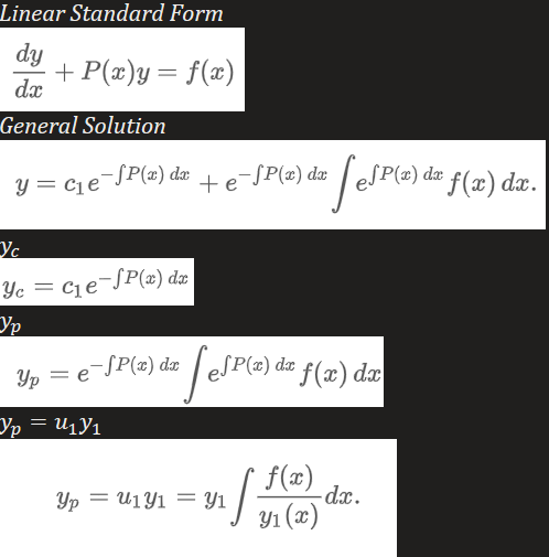
Linear 1^st-Order (Possible Exam Question)

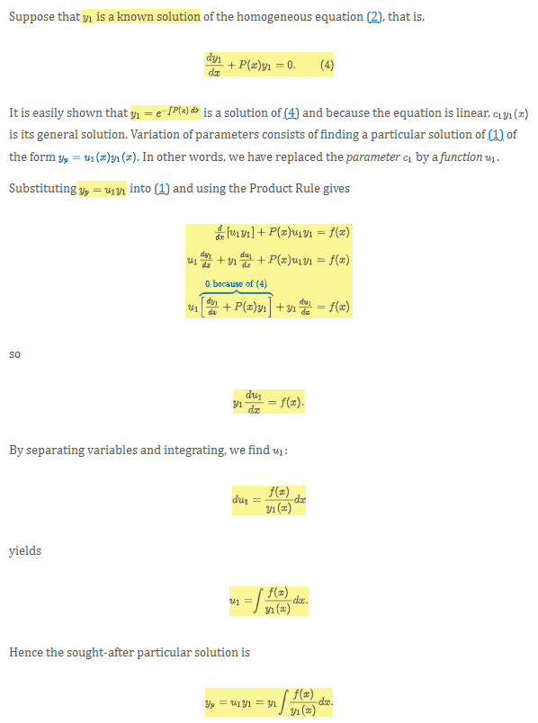
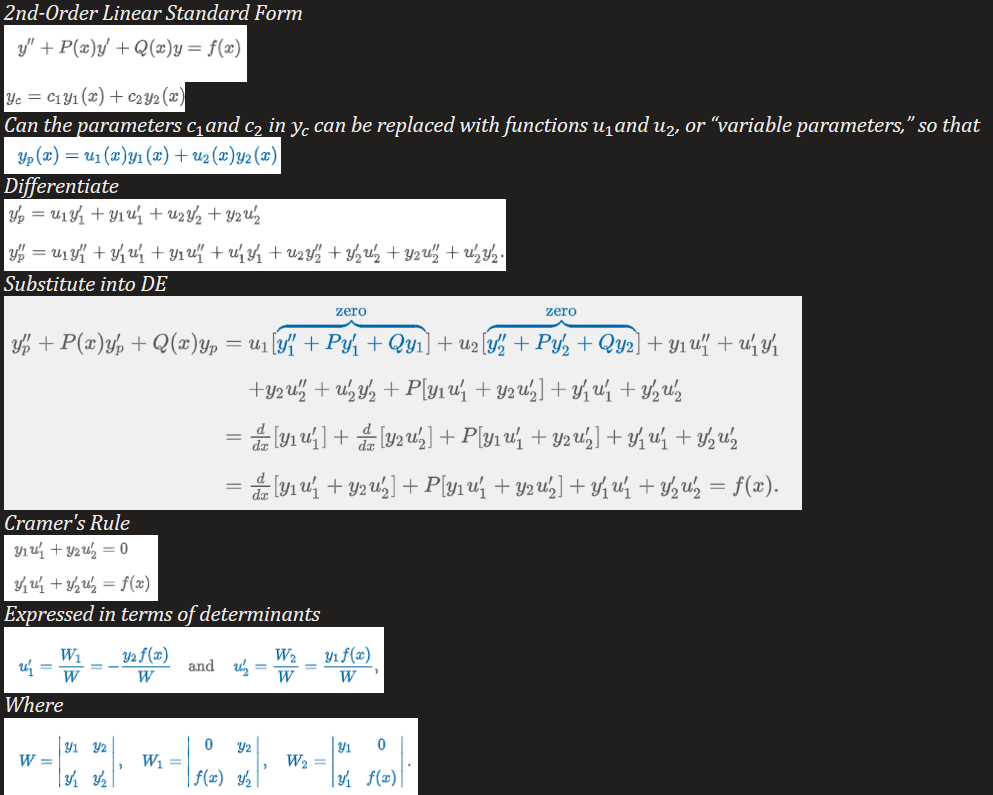
Variation of Parameters

Note: do not need to introduce new constants, solution method may involved integral-defined functions, particular solution may not be unique

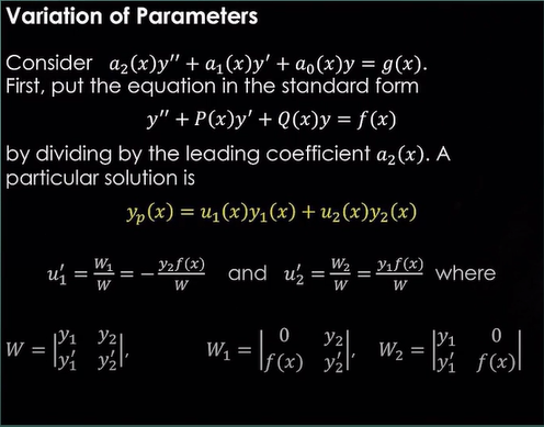
Variation of Parameters Proof of Linear 2^nd-Order (Possible Exam Question)

Note: can be generalized to linear n^th-order equations that have been put into standard form

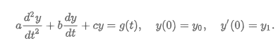
Linear Dynamical System

y(0) = y₀ & y’(0) = y₁: Initial Conditions w/ t=time

g(t): Driving function/Forcing Function/Input

Solution y(t): Response/Output

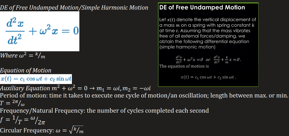
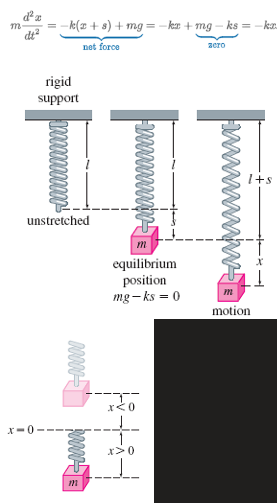
Spring/Mass System: Free Undamped Motion

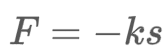
Hooke’s law

“spring exerts a restoring force F opposite to the direction of elongation and proportional to the amount of elongation s”

k > 0: constant of proportionality called the spring constant or stiffness of the spring

Newton’s 2^nd Law

m(d²x/dt) = -k(x + s) + mg = -kx +mg - ks = -kx

F₁ = -k(x+s) : restoring force

W = mg: Weight = mass*acceleration

• mg = ks or mg -ks = 0: condition of equilibrium (stretched- elongation/compression)

• x(t): displacement where x = 0 is the equilibrium position, above is negative, below is positive

• F = ma: Force = mass* acceleration

• a = d²x/dt²: acceleration

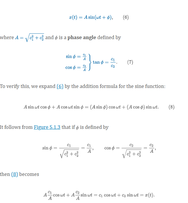
Free Undamped Motion - Alternative Form of x(t)

amplitude A

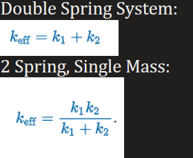
Effective Spring Constant

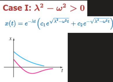
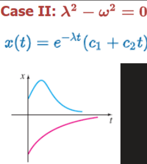
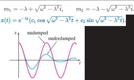
Spring/Mass Systems: DE of Free Damped Motion

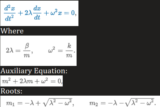
Case 1: Overdamped

Case 2: Critically Damped

Case 3: Underdamped

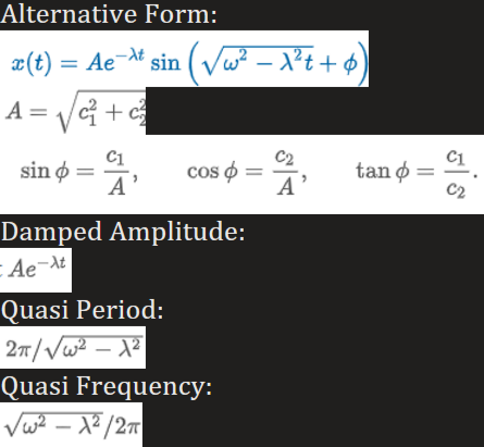
Free Damped Motion - Alternative Form of x(t)

amplitude A

Spring/Mass Systems: Driven Motion with Damping

Take into consideration an external force f(t) acting on a vibrating mass on a spring.

• Note: when F is a periodic function, it is considered a transient term; in other word, y_c = transient term, y_p = steady-state term

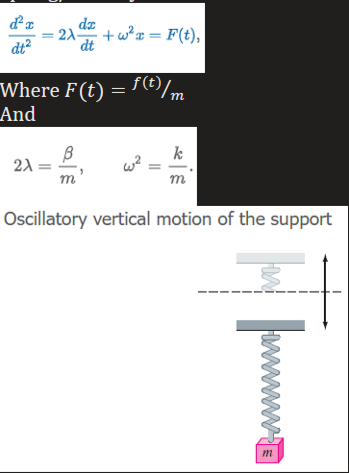
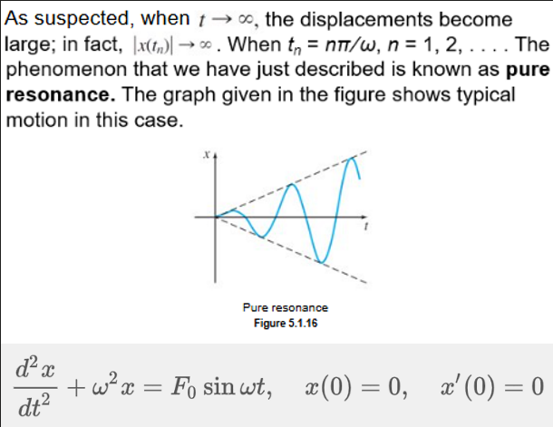
Spring/Mass Systems: Driven Motion without Damping

With a periodic impressed force and no damping force, thereis no transient term in the solution of a problem. ​

Pure Resonance

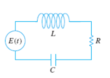
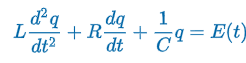
LRC Series Circuit

“Kirchoff’s 2^nd Law states the impressed voltage E(t) in a closed loop equals the sum of the voltage drop.”

E(t) = impressed voltage ~ external force, f(t)

i(t) = current in closed circuit

q(t) = charge incapacitor at time t

L = inductance ~ mass, m

R = Resistance ~ damping constant, b

C = Capacitance ~ spring constant, k

• E(t) = 0: electrical vibration of the circuit are free

• E(t) > 0: electrical vibrations are forced

  • R ≠ 0, q_c(t) = transient solution, q_p(t) = steady-state solution

• general solution contains the factor e^-Rt/2L

• the capacitor is charging and discharging as t→∞ (simple harmonic)

• E(t) = 0 & R = 0: undamped, electrical vibrations fo not approach 0 as t increases without bound