Lecture 04: Populations l

A population

is a group of individuals of the same species, living and interacting with one another in a particular area).

Abundances

numbers of individuals

Densities

numbers of individuals relative to the area they occupy of natural

Abundances and densities of populations change all the time.

• Understanding population growth is necessary in many fields, including conservation, human demography, epidemiology, and medicine

• Covid cases growth, growth of a tumour

Censusing a population can be challenging. What do you count?

• Different individuals in a population can vastly differ in their characteristics (e.g., male vs female) and/or abundance (e.g., juveniles vs adults).

• Substantially different abundance estimates can be obtained depending on what is included in the count, which in turn, is determined by a study’s objectives (e.g., it might be sufficient to only count reproducing individuals)

Censusing a population can be challenging. Where do you count?

• Defining a population’s boundaries could in some cases be straightforward (e.g., due to natural geographic barriers, such as on islands), and in other cases be unclear (e.g., in highly mobile species with large home ranges).

• Studies of movement, genetics, and other factors can inform on natural population boundaries, but often educated guesses need to be made regarding these boundaries and whether a population is open (substantial immigration and/or emigration) or closed (no immigration or emigration).

Censusing a population can be challenging. How do you count?

• Counting all individuals in a population is usually impossible.

• Researchers must rely on counting representative subsamples of a population, and then extrapolate from that subsample to get an estimate of total population size

• For example, if density does not vary across the entire population area, then we can estimate total population size by estimating density in a representative area, and then extrapolating to the total population area.

• Ntotal / Atotal = Nsamples / Asamples

Multiple methods exist for censusing populations.

• The approach and its accuracy will vary between species and contexts and is also often influenced by logistic constraints.

• Counting sight of species

• reports by the community, such as from trappers and hunters

• sampling plots for sessile species

• line transects by sight or sound for mobile species

• mark-recapture methods

counting signs of species

• this approach can be particularly useful for cryptic species, but typically only yields estimates of relative abundance (e.g., the number of animal tracks in an area).

• These can correlate with absolute population size, but this may not always be the case (e.g., differences in the number of animal tracks among two areas may reflect differences in abundance AND/OR differences in activity).

through reports by the community, such as from trappers and hunters

while such reports are essential for sustainable management and can in some cases yield outstanding data (e.g. Lecture 1: lynx-hare population cycles), they typically include “sampling” biases that would not be present in scientific surveys (e.g., hunter preferences for larger animals)

sampling plots for sessile species

• Sample part of population and extrapolate to everywhere else

• Good for things that don’t move, like coral reefs

line transects by sight or sound for mobile species

• Common for animals that are hard to capture like elephants, sharks, birds

• Let’s say im trying to figure out how many birds are in an area, and i have no idea that its 1000 birds

• Im gonna go for a walk and make note everytime i see a bird

• At the end of the walk you say ‘’this is how many birds I walked when I walked this far, at this speed, the birds were this distance away from me”

• The logic is if there were larger population I will see more birds. If its a smaller population I would see less birds

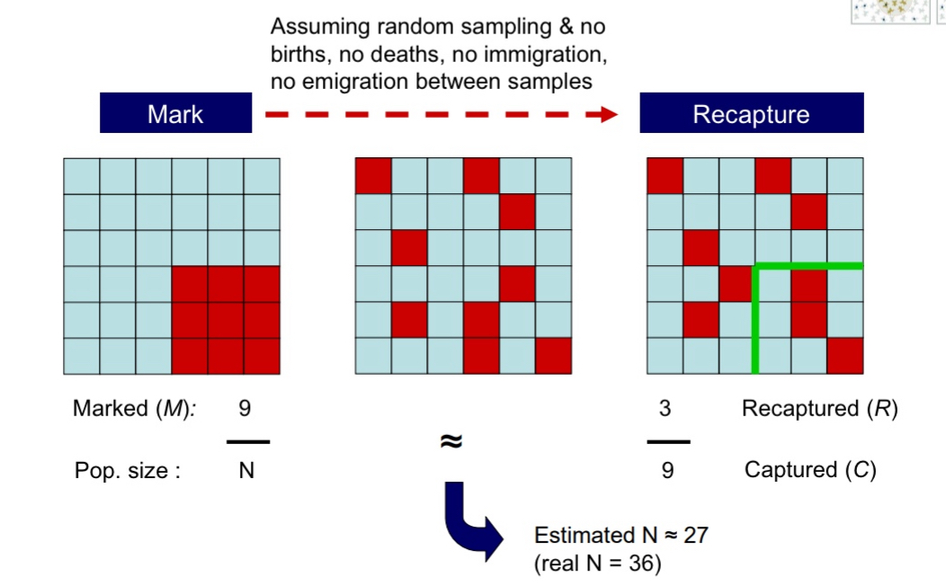
mark-recapture methods

• Only use for animals you can distinguish from each other (won’t use for pumas because they are indistinguishable.

• Use collars with signals that will give the researcher the specific info (like case number) of that individual, or use trackers and banding → when I recapture the animal I will know exactly which animal that was

• Proportion of individuals marked in total population = proportion of individuals marked in second sample

• Solve for N for an estimate

• Larger the population size, or the more often you do this, the better the estimate will be

mark-recapture methods On orsolot

• Like finger prints, the pattern on their fur is different for each individual → don’t need trackers or bands because the fur gives away which individual is which

• Here, a random subset of individuals is captured and marked/tagged, then released. At a later date, the population is sampled again; the ratio of marked to unmarked individuals in the sample can be used to estimate population size.

• Mark-recapture techniques can often be used for abundance estimates, regardless of whether or not the animal is physically captured, for example, by using camera traps.

• Recaptures of individual cats are identified based on fur coat pattern → data of “i saw this individual in this specific location. Recaptures history can tell me a number of things”

Camera traps can tell us

• data of “i saw this individual in this specific location. Recaptures history can tell me a number of things” → abundance

• Since we are physically seeing the animals, we can see things like deformities (blind in one eye) or scars that might hinder their performance (can’t see prey and catch food good enough) and overall quality of life

  • Condition of animals as a whole like what diseases are present

• What habitats are certain animals using based off where the animal was recorded

• Species diversity → community level → what species are present, how many of each are present → differing levels of biodiversity (closer to humans you get, biodiversity goes down)

• Proportion of adolescence vs adults → basic demographics (population growth, are there enough young and old, males and females)

• Look at competition of different species for resources → causes separation especially when one species beats the other species and gets the resources every time.

  • Species interactions

• How does animal behaviour change when it comes to different weather patters, or time of days (ie animal is nocturnal)

• Find out when the reproduction season occurs, and how many offspring can an animal reproduce at once / in one season

• Predator prey associations

• Mortality → if i don’t see an individual, can I tell if they just left the area or dies (use data like their age and estimated life expectancy to differentiate)

• Movement patterns

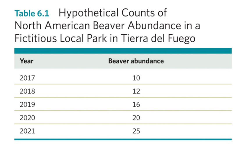
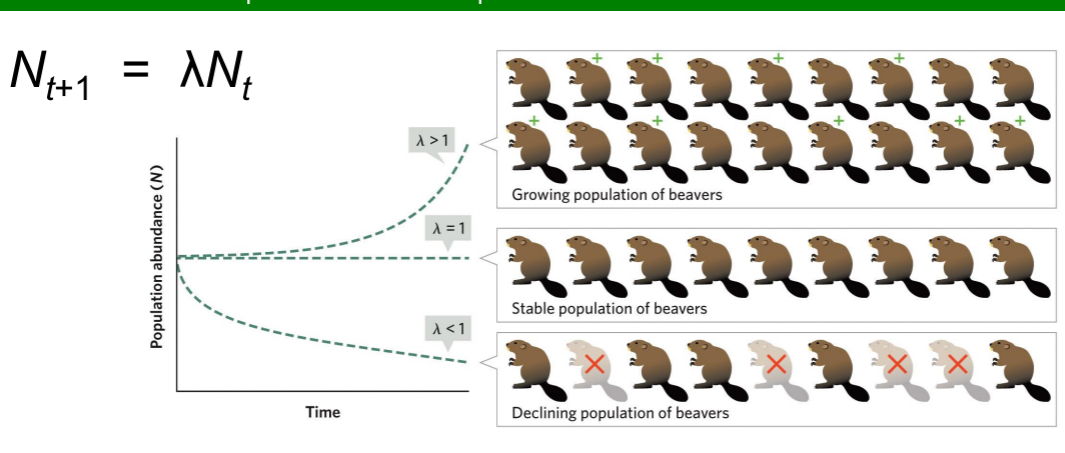
Population Growth Example: Beavers in Tierra del Fuego, Argentina

• Beavers were brought there, so that humans could hunt them. But in Argentina, beavers don’t have any predators. So they build dams with the wood from trees. They throw off the entire ecosystem because beavers are not native

• To manage the beaver population, regular population censuses might be conducted.

• A manager must then use these data to estimate population growth rates and future population sizes.

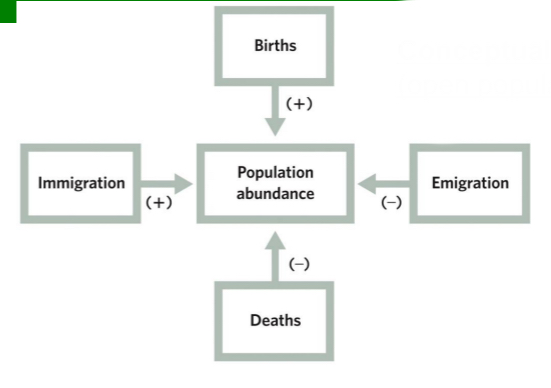
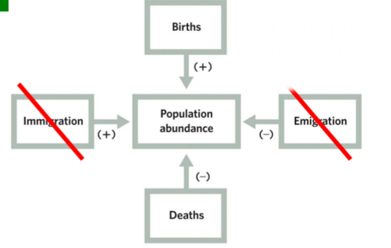
Population abundance at time t+1

will equal population abundance at time t plus all individuals that were added to the population between t and t+1 minus all individuals that were lost from the population between t and t+1.

Mathematical Model (open population)

• There is immigration and emigration

• Nt+1 = Nt + Bt - Dt + It - Et

  • Nt+1 = pop. size (at time t+1)

  • Nt= pop. size (at time t)

  • Bt= no. of births(between times t and t+1)

  • Dt= no. of deaths (between times t and t+1)

  • It = no. of immigrants (between times t and t+1)

  • Et = no. of emigrants (between times t and t+1)

Mathematical Model (closed population)

• Nt+1 = Nt + Bt - Dt

  • Nt+1 = pop. size (at time t+1)

  • Nt= pop. size (at time t)

  • Bt= no. of births(between times t and t+1)

  • Dt= no. of deaths (between times t and t+1)

• Populations may be open (substantial immigration and/or emigration) or closed (no immigration/emigration).

Open populations can sometimes be treated as closed for population assessments

e.g., if the number of immigrants equals the number of emigrants, or if immigration and emigration are small compared to the total population abundance.

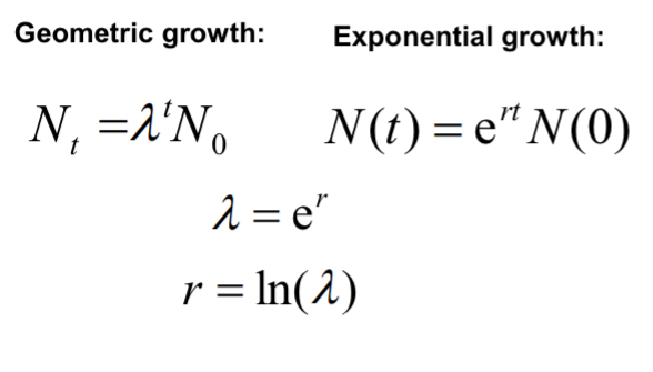
The Geometric Model of Population Growth

• The terms Bt and Dt in our population growth model may depend on many factors, including environmental conditions and population size.

• For a first, simple model, let’s assume that the per capita birth rate and the per capita death rate (specifying the average number of births per individual per time unit and the average probability of death per individual per time unit, respectively) are constant and do not vary with environmental conditions or population size.

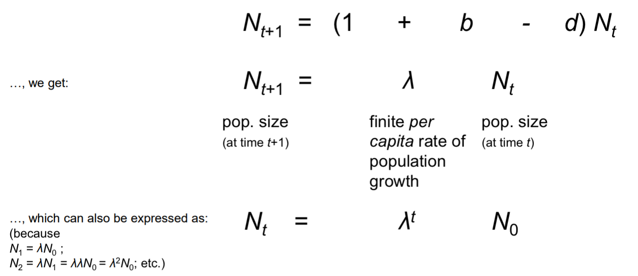
• Nt+1 = Nt + bNt - dNt

  • Nt+1 = pop. size (at time t+1)

  • Nt= pop. size (at time t)

  • bNt = per capita birth rate, b, times pop. size (at time t)

  • dNt = per capita death rate, d, times pop. size (at time t)

Simplifying… Nt+1 = Nt + bNt - dNt

Properties of λ

• A population grows when individuals produce on average more than one offspring during their lifetime.

• When λ = 1, population size stays the same.

• When λ < 1, population size declines geometrically.

• When λ > 1, population size increases geometrically.

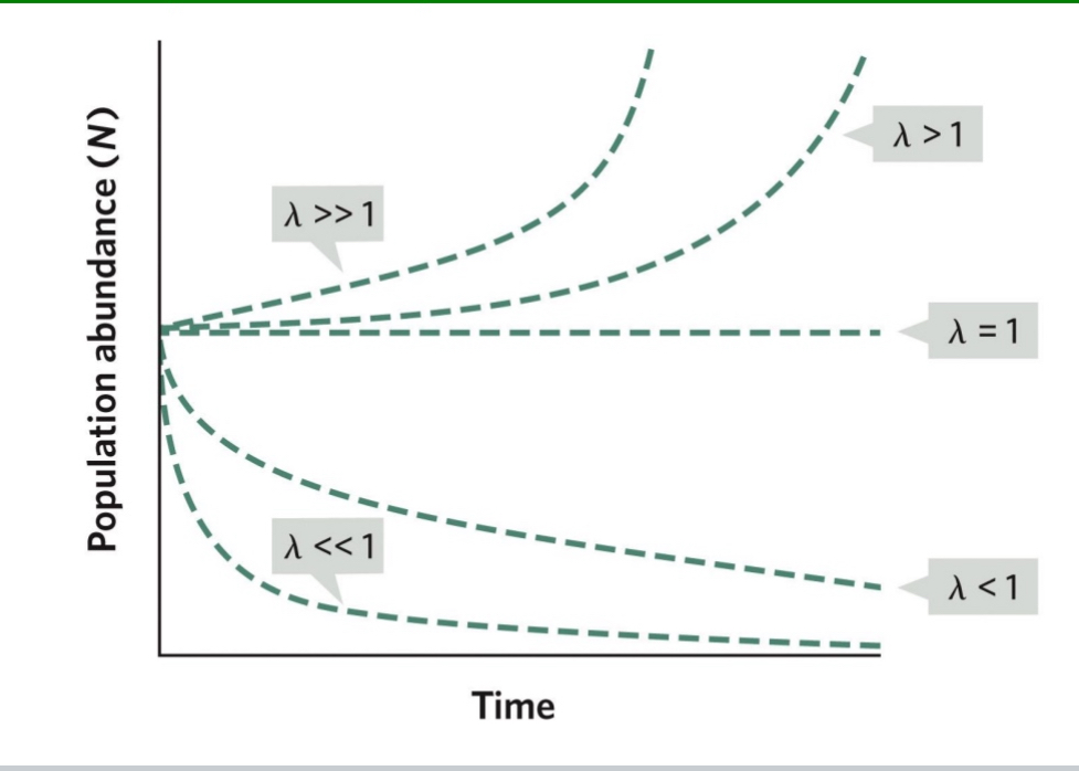
When λ = 1

population size stays the same.

When λ < 1

population size declines geometrically.

When λ > 1

population size increases geometrically.

λ Graph → magnitude differences

Larger λ → faster population growth

Estimating Annual Population Growth Rates

• Using the geometric model of population growth, Nt+1 = λNt, and rearranging the equation to λ = Nt+1/Nt , we can estimate the annual finite per capita rate of population growth for a given population from subsequent years of data.

• In yrs 2018/19→ 16/12 =33%

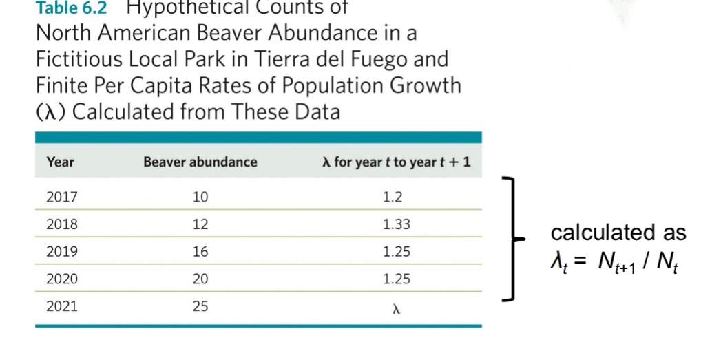
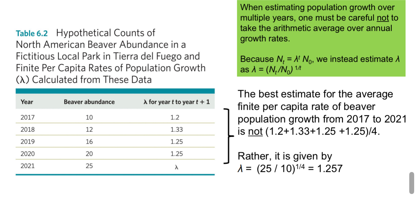
Estimating Population Growth Rates over Multiple Years

• When estimating population growth over multiple years, one must be careful not to take the arithmetic average over annual growth rates.

• Can’t take the average

• Because Nt = (λ ^t) N0, we instead estimate λ as λ = (Nt /N0) ^ 1/t

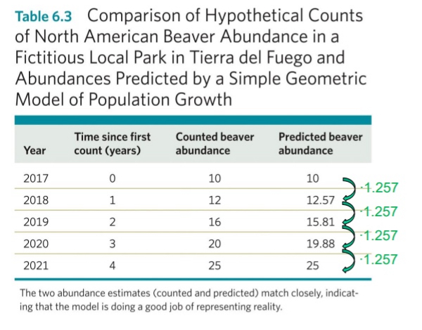
Population Projections

Using the geometric model for population growth, Nt = λ ^t N0, and an estimate of λ and initial population size N0, we can project how large the population would be t time steps into the future, if the model’s assumptions remain fulfilled.

Assumptions of the geometric model of population growth:

• closed population

• changes in population abundance are concentrated around a discrete time period (e.g., breeding season)

• per capita birth and death rates are independent of the environment or population size

• all individuals are treated equal; there is no distinction between adults and juveniles or males and females

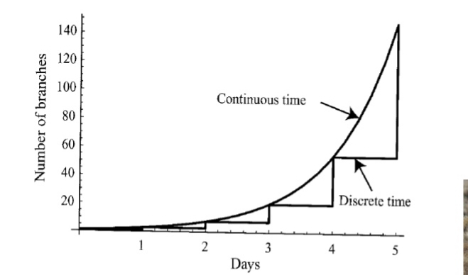
Discrete-time population models

• aim to track population size from time step to the next.

• They are most appropriate for species / situation where large changes in numbers occur periodically at a specific time point, such as during birth pulses in annually reproducing animals.

• calculate population size at the next time step as a function of population size at the previous time step

Discrete-time population models Formula

• N t+1= f(Nt) = Nt + increase - decrease

  • N t+1 = pop. Size at time t+1

  • f(Nt) = function of pop size at time t

Continuous-time population models

• for population changes instantaneously, and are most appropriate for species where population abundance changes continuously, such as in continuously reproducing species

• calculate population size for all times t based on a starting condition and the rate of change as a function of population size

Continuous-time population models Formula

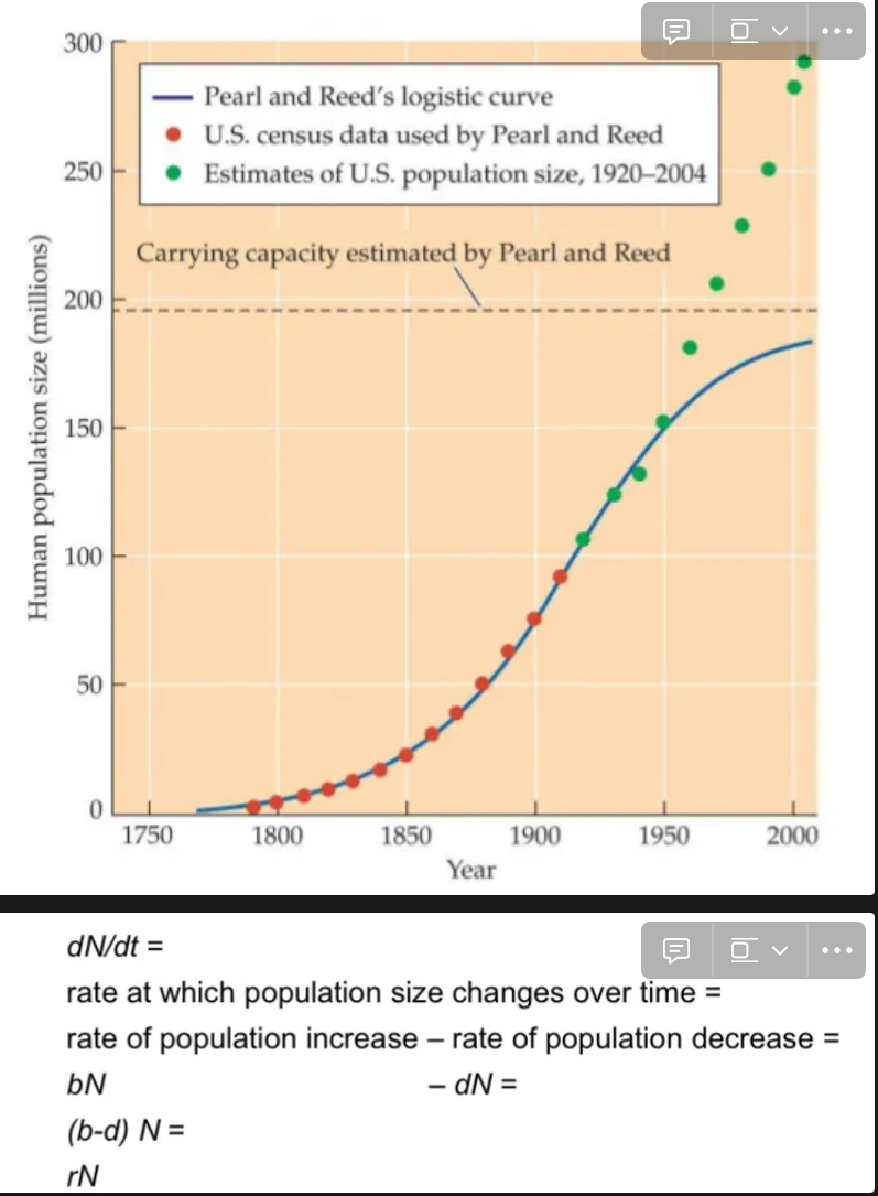
• dN/dt = f(N) = rate of increase - rate of decrease ; N(0) =N0

  • dN/dt = rate of change in population size (at time t)

  • f(N) = function of pop size at time t

  • N(0)=N0 = initial population size (at time 0)

Discrete-time population models Vs Continuous-time population models

If f(N) > 0

the population increases (the larger f(N), the larger the rate of increase).

If f(N) = 0

the population does not change.

If f(N) < 0

• the population decreases.

• (the smaller f(N), the larger the rate of decrease).

Exponential growth

• occurs when individuals reproduce continuously rather than at discrete time periods (e.g., humans) and when the growth rate does not change over time.

• dN/dt = rN

  • dN/dt = rate of change in population size at each point in time (=derivative of N(t))

  • r = intrinsic per capita rate of increase

• rate at which a population changes (Ieft-hand side) is proportional to population size (right-hand side). If r does not change over time, the population increases exponentially because the total rate of change increases with population size

• N(t) = N(0)e^(rt)

  • Solve for N(t)

Geometric and exponential growth curves overlap

because the equations are similar in form. λ can be calculated from r, and vice versa.

r = 0

population size stays the same.

r < 0

population size declines (exponentially).

r > 0

population size increases (exponentially).

Differential equation models do not look intuitive at first glance. Why bother?

• Let’s say your goal is to describe human population growth with an equation

• N(t) = …

• The problem is that it is not intuitively clear what this equation should look like.

• Example: Would you have guessed (without any knowledge of the logistic equation) that the following might be a good description of population growth?

• Solution: Even though it might not be possible to directly write down an equation N(t) = …, it is usually possible to write down an equation for the rate of change as a function of the processes determining that rate of change, and then solve the equation for N(t). E.g., density-independent growth, where the rate of change depends directly on the rates of birth and deaths:

Density-Independent vs Density-Dependent Population Regulation

• The geometric and exponential models of population growth both assumed that per capita birth and death rates stay constant over time.

• In reality, both per capita birth rates and per capita death rates will vary both with density-independent and density-dependent factors.

Density-independent factors

• are factors that affect birth rates, death rates, and other demographic variables independently of how many individuals there are in a population (e.g. weather conditions, catastrophes…

• Have nothing to do with population

• Ex. Population of 1000 elk, then a big forest fire. A bunch of elk die. That has nothing to do with the fact that there was 1000 elk. If there were 100 elk, they would die. If there were 10 elk, those 10 elks would die

• Eg. Lightening struck a herd of reindeer. If there were 10, 100, 10000, they would all die regardless of how many there are.

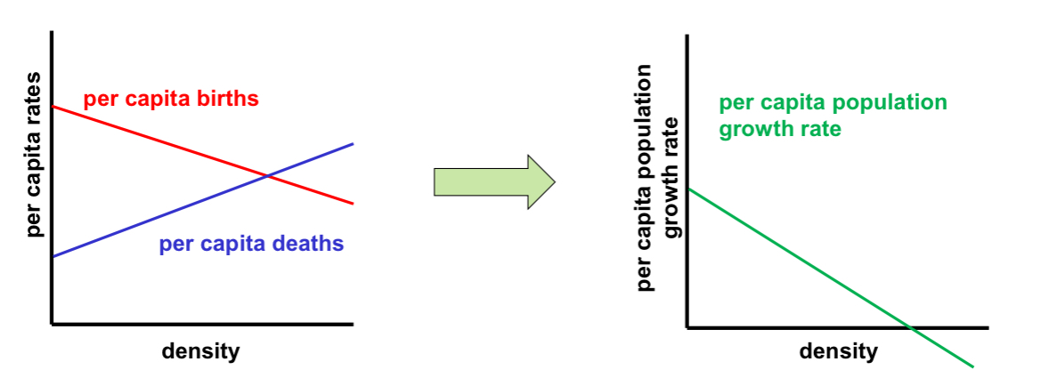
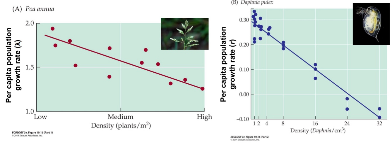
Density-dependence

• occurs when birth rates, death rates, and/or other demographic variables are directly affected by the density of the population.

• This is because they start competing for resources that aren’t enough for everyone in the population

• Ex. Put bacteria in Petri dish, give them food, they start growing. At some point they will reach limits of the dish and there is do were else to go.

  • Death will increase, reproduction will decrease, or both

• e.g. density-dependent reproduction: (birth rates generally tend to decrease with increasing density)

• E.g density-dependent mortality: (mortality rates generally tend to increase with increasing density)

• e.g. density-dependent dispersal: (dispersal rates (i.e. emigration) generally tend to increase with increasing density)

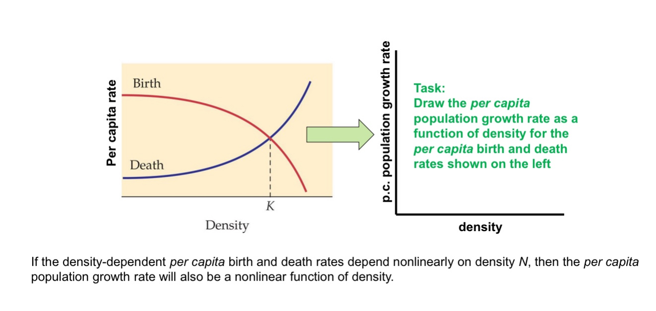
• e.g., if there is no immigration and emigration, and if the per capita birth rate decreases linearly with density and the per capita death rates increases linearly with density, then the per capita population growth rate (e.g., r(N) = b(N) – d(N) in the exponential growth model) decreases linearly with density

In density dependence: if densities become high enough to cause λ = 1 (in the geometric growth model) or r = 0 (in the exponential growth model),

the population stops growing; if λ < 1 (r < 0), the population declines.

Solve this red line - blue line