ST 311

ncsu

Data

Collections of observations (measurements, counts, and survey responses)

Population

Complete collection of all measurements or data that is being considered. Aka population of interest

Sample

A subset of members selected from a population

How to select a sample

Should be random and representative of the population

Parameter

Numerical measurement describing some characteristic of a population

Statistic

Numerical measurement describing some characteristic of a sample

Quantitative Data

aka numerical data; consists of numbers representing counts or measurements

Examples of quantitative data

age of an athlete, weight of a letter

Categorical Data

aka qualitative data; consists of names or labels

Example of categorical data

college major, hometown

Discrete Data

result when the data variables are quantitative and the numbers are countable/finate

Example of discrete data

the number of tosses of a coin before getting tails

Continuous/numerical Data

result from infinitely possible values, uncountable

Example of continuous/numerical data

the arm span of high school seniors

Bias

those samples that are more likely to produce some outcomes than others (resulting statistics might be too high or too low)

Convenience

those samples that are easy to collect (often have some bias or don’t represent the population in general)

Volunteers

a self-selected sample of people who respond to a general appeal

Simple random sample

a sample of x subjects is selected in such a way that every possible sample of the same size n has the same chance of being chosen

Stratified sample

subdivide the population into at least two different groups, so that the subjects within the same subgroup share the same characteristics. then draw a sample from each subgroup

Cluster sample

divide the population area into naturally occurring sections then randomly select some of those clusters and choose all members from the selected cluster

Systematic sample

select some starting point and then select every n^th element in the population. works well when units are in some order (ex. house on the block)

Multistage sample

collect data by using some combination of the basic sampling methods

Bad sampling frame

when attempting to list all members of a population, some subjects are missing. can be difficult to obtain a complete list

Undercoverage

the sampling frame is missing groups from the population

Non-response bias

some parts of the population chose not to respond

Response bias

responses given are not truthful

Wording/order

wording of questions is leading to elicit a particular response

Experiment

the process of applying some treatment and then observing its effects. almost always compares two (or more) groups (treatment vs control)

Observational study

the process of observing and measuring specific characteristics without attempting to modify the individuals being studied. tells what’s happening and cannot describe cause-effect relationships

Response variable

measures an outcome of a study

Explanatory variable

explains or influences changes in the response variable

Treatment effects

different treatment = different outcome (what we want)

Experimental error

variability among observed values of the response variable for experimental units that receive the same treatment

Lurking variables

a variable that is not among the explanatory variables in a study and yet may influence the interpretation of the relationship among response and explanatory variables

Confounding variables

two variables are confounded when the effects on the response variable cannot be distinguished from each other

Control

control the effects of lurking/confounding variables by careful planning (control group receives no treatment)

Randomization

randomly assign experimental units to treatments to reduce or eliminate bias

Replication

measure the effect of each treatment on many units to reduce chance variation in results

Completely randomized design

participants are randomly assigned to treatments (including control group). Assumes that on average lurking variables will affect each treatment group equally

Randomized block design

divides participants into subgroups called blocks. Variability within blocks is less than variability between blocks. Participants from each block are then randomly grouped.

Matched pairs designed

used when an experiment has only 2 treatment groups; participants can be grouped into pairs and within pairs are randomly assigned to different treatments

The placebo effect

the tendency to react to a drug or treatment regardless of its actual physical function.

Hawthorne effect

behavior is different because the subject knows they are being watched

Blinding

When individuals associated with an experiment are not aware of how subjects have been assigned

Single blind study

those who could influence the results are blinded

Double blind study

those who evaluate the results are blinded as well

Measure of center

a value at or near the middle of a data set (mean, median, mode)

∑

denotes a sum, “sigma”

x

denotes an individual data value

n

denotes the number of values in a sample, “sample size”

N

denotes the number of values in a population

x̅

denotes the sample mean, “x bar”

μ

denotes the population mean, “mew”

Mean

found by adding all values and dividing by the number of values in a data set (uses every data value so not good for skewed data)

Median

the value in the middle when listed in ascending order (not affected by outliers, can be used with any data set)

Mode

the value that occurs with the greatest frequency (only useful for multimodal or qualitative data)

Unimodal

dataset with one mode

Bimodal

dataset with two modes

Multimodal

dataset with more than two modes

Which measure of center do you choose?

Quantitative = mean or median

Categorical = mode

Horizontal histogram

represents quantitative data

Vertical histogram

represents frequency

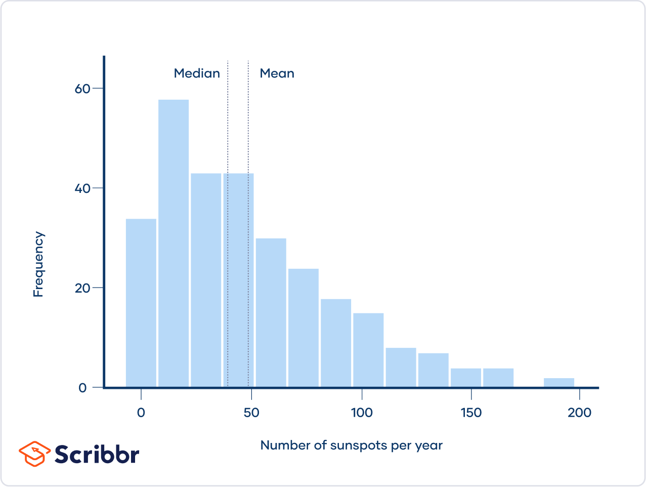
Right skewed histogram

highest amount to the left

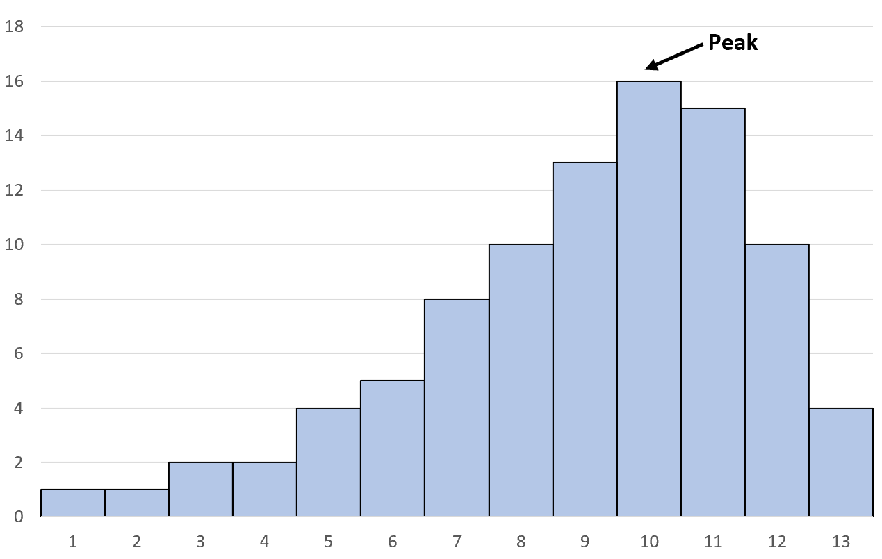
Left skewed histogram

highest amount to the right

Symmetrical

mean = median = mode

Right skewed (pos)

mode < median < mean

Left skewed (neg)

mean < median < mode

Range

the difference between the maximum and minimum

R = max value - min value (highly affected by outliers)

Interquartile range

provides a range of values that are not as affected by potential outliers

IQR = Q₃ - Q₁

Varience

V = (standard deviation)²

Standard deviation

SD = √V

Standard deviation

a measure of how much data values deviate from the mean. Increases with 1 or more outliers (never negative)

σ²

population variance

σ

standard deviation

s²

sample variance

s

standard deviation

z-Scores

when you want to compare two numbers from different groups relative to their own groups

Positive z-score

data value is above average

Negative z-score

data value is below average

z-score equation

Z=\frac{x-\mu}{\sigma} (value - mean / standard deviation)

-1 \sigma  to +1 \sigma  

68% of the data lie between these

-2 \sigma to +2 \sigma

95% of the data lie between these

-3 \sigma to +3 \sigma

99.7% of the data lie between these

The emperical rule

for a normal distribution, approximately 68% of data falls within 1 standard deviation of the mean.

Significantly low

values are considered significantly or unusual if they are -2 \sigma  or lower

Significantly high

values are considered significantly or unusual if they are +2 \sigma or higher

Probability

represented by the area under the density curve

Normal distribution (total area under the curve is equal to 1)

a continuous probability distribution for a random variable. Mean, mode, and median are equal. Bell-shaped and is symmetric about the mean.

Parameters

The mean is located in the center and the standard deviation defines the shape

Normal distribution

X~N( \mu  , \sigma )

The standard normal distribution

the distribution of z-scores, has a mean of zero, and a standard deviation of one.

Z~N(0,1)

Probability distribution

describes how likely the values of the variable are to occur

Binomial distribution

a binomial random variable counts the number of successes that must be true

Qualities to make a distribution binomial

1. Fixed number of trials/observations labelled as “n”

2. Independent trials (outcome of one doesn’t affect the probability in the others)

3. Either a success (S) or failure (F)

Success in binomial distributions

when the outcome that a random variable is counted, probability of success is constant for each trial.

Success equation

P(S) = p

Binomial equation

X~B_in(n, p)

n = # of trials & p = probability of success

Mean of binomial distribution

\mu=n\cdot p  (the mean of a random variable, aka E(x), the expected value)

E(x)

the expected value, a weighted mean of the outcomes (likely outcomes get more “weight” than unlikely)

Expected value vs mean of random variable

expected value of a discrete random variable is equal to the mean of the random variable