Forecasting

Ljung-Box Degree of Freedom

ARIMA: dof = p+P+q+Q

Dynamic Regression: dof = lags - p - q

Seasonal ETS: dof = 0

Non-Seasonal ETS: dof = n smoothing params

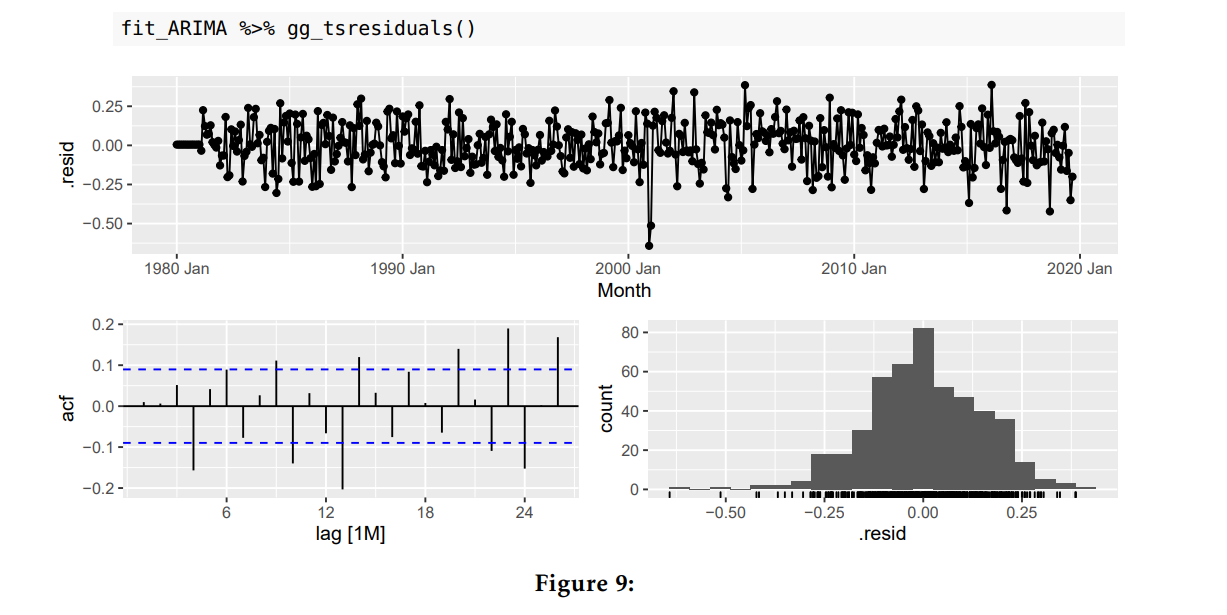
Innovative Residuals should be I.I.D

Use the ACF to determine whether there is time dependnece and hence prove if residuals are independant. (5% rule)

Use Time/Residual plot to determine whether residuals are homoscedastic and ensure there is no pattern to confirm they are identical

Use Histogram to determine whether residuals are normally distributed. The plot should be unimodal with no wide tails.

Should we always use AIC?

• This is almost true.

• The AICc is very useful and we prefer to use it when possible, as it uses all the sample and is asymptotically equivalent to minimizing one-step time series cross validation MSE assuming Gaussian residuals.

• However it is limited and cannot be used when comparing across different classes of models or even sometimes within the same class (for example ARIMA models with different orders of differencing, or models with different transformations).

Describing Timeplots

Trend: Is it present? Is it localised or global? is it additive or multiplicative. If localised, where is it increasing, where is it decreasing?

Error: Is the data heteroskedastic? Are fluctuations irregular?

Seasonality: What is the seasonal period? Is the seasonality additive or multiplicative? Does the seasonality change?

Cycle: Is there structural breaks? Are cycles present, if so where are they occuring, and why?

Describing seasonal plots

Benefit: Tells us the seasonal shape

Describing subseries plots:

Benefit: Tells us the seasonal averages

Example: Describe the patterns in the time-series plot

• the time plot shows a long-term/global upward trend, hence the number of births have overall grown over time.

• the time plot shows that the series has cyclical features, peak around 1990-1991, trough around 2001-2002 and another downturn starting around 2016.

• the time plot shows constant seasonal variation throughout the sample, i.e., additive seasonality.

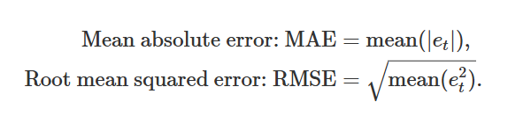
Scale Dependant Errors

ME the mean of the error.

RMSE It measures the average difference of the actual data points from the predicted values, and the difference is squared to avoid the cancelation of positive and negative values, while they are summed up.

MAE the absolute mean of the error

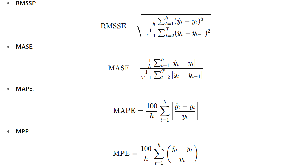
Scale-independant errors

Allow us to compare different time series on different scales (e.g cm vs meters)

MAPE

MASE (Mean Adjusted
MPE (Mean Percentage Error)

RMSSE

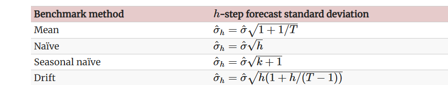
h-step ahead forecast standard deviation for benchmark models

See image

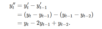
What is y’’t

The second order difference

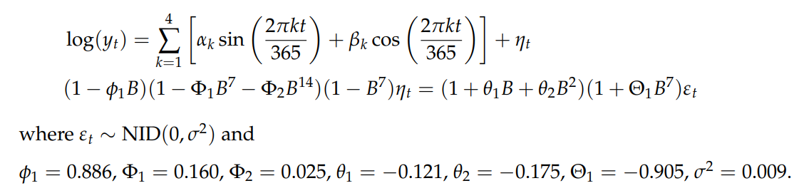
Write down the dynamic regression model, with log transformation and ARIMA error term using backshift notation.

Ensure you state how the error term is distributed.

See image for solution

R autoselection chooses models which minimise AICc, why is this appropriate?

Selecting models based on minimising the AIC (or AICc which corrects for small samples) assuming Gaussian residuals is asymptotically equivalent to minimising one-step time series cross validation MSE. Hence, this focuses on forecasting.

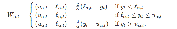
Explain how the winkler score can be used to assess the distributional accuracy of a forecast confidence interval

The Winkler score Wα first applies a penalty based on the width of the prediction interval where α is the level of significance considered. This is reflected by (uα − ℓα). Hence, the 1 wider the prediction interval the higher/worse the Wα. If the prediction interval contains the 1 observed value then Wα = (uα − lα). If the observed value is outside the prediction interval an 1 additional penalty is applied proportional to how far the observation is outside the interval. If the observation is below the lower bound the additional penalty

Explain the process of time-series cross vlaidaiton

• TSCV involves fitting models to multiple training sets 1 • If available data is y1, . . . , yT, then training sets are expanding of the form y1, . . . , yt , where t = p, p + 1, . . . , T. 1 • Initial training set of size p where p chosen to ensure a model can be estimated. 1 • Evaluation on yt+h for a specific h and all t.

An ETS model for Holt’s linear trend method, is a generalisation of an ETS model for simple exponential smoothing. It should therefore always be preferred as it will produce better forecasts.

This is not true. 1 • Yes ETS(A,A,N) is a generalisation of ETS(A,N,N). 1 • However the generalisation involves estimating an extra smoothing parameter and an extra initial state for the slope. 1 • An information criterion, such as the AICc, will penalise the fit of the model for the extra degrees of freedom

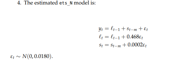
Write the ETS(A,N,A) model using an observation and state space equaiton from the ouput

see image

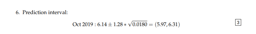
What is the one step ahead 80% confidence interval for the ETS(A,N,A) model

see image

ETS vs ARIMA

• These model classes are not interchangeable. 1 • Some of the simpler additive models are equivalent including SES and Holt’s method with additive errors. 1 • ETS models with multiplicative errors handle heteroskedasticity, whereas ARIMA models do not. 1 • ARIMA models handle a much wider range of dynamics than ETS models. 1 • ETS models cannot be used for stationary series.

STL Analysiss

• ensure windows are an odd number, so that smoothing via moving averages is centred.

• ensure the error component not random, if it error component has seasonal behaviour then the seasonal window may be set too high.

• ensure each component is not too spiky, we want to see the overarching trends, etc. If we set our window too small we may be capturing random noise instead of a meaningful signal.

• If the data has outliers consider robust to outliers setting.

ETS Vs ARIMA

• These model classes are not interchangeable. 1 • Some of the simpler additive models are equivalent including SES and Holt’s method with additive errors. 1 • ETS models with multiplicative errors handle heteroskedasticity, whereas ARIMA models do not. 1 • ARIMA models handle a much wider range of dynamics than ETS models. 1 • ETS models cannot be used for stationary series.

Confidence Interval size & uncertainty

We want our prediction intervals to have as close as possible to the correct coverage, without that defining whether they are narrower or wider. 2 • Usually prediction intervals will have lower coverage than what they aim for, i.e., they will be narrower, as they do not account for all sources of uncertainty, e.g., they do not account for the uncertainty

Regression models assumed seasonal and trend patterns are fixed → they may underestimate uncerainty and produce overly small confidence intervals.

ETS Models are generally overly confident and produce too narrow intervals, especially in the long-term. They also do not consider previous cyclic behaviour in uncertainty.

• SNAIVE confidence intervals are fixed, naive confidence intervals grow.

ARIMA models will produce inaccurate coverage of confidence intervals when multiplicative seasonality is present.

For backshift notation, which components do we subtract from 1, which do we add.

(1-phi)

(1+theta)

Long-term behaviour

• Dampened trend ETS methods will flatten out in trend, seasonality remains consistent

• ARIMA values will often flattedn out and approach a constant.

• Regression models assume seasonality and trend is deterministic - therefore may not account for chaing trend.