CSC 345 Big Data and Machine Learning

Scalar

A single number, usually written in italics, named with a lowercase variable name. When first introduced it should be specified what kind of number they are. e.g. let

n ∈ N

be the number of units.

Vector

An array of numbers, arranged in order. Typically given a lowercase variable in bold name such as x,where the first element is x₁.

They should be thought of as identifying a point in space, with each element giving the coordinate along a different axis.

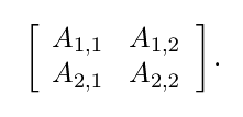
Matrix

A 2D array of numbers, where each element is identified by two indices rather than one. Normally given uppercase, bold variable names such as A. If A has a height of m and a width of n, then we say that A ∈ R^m×n.

We can identify all the numbers with vertical coordinate i by writing a “:” for the horizontal coordinate. For example, A_i,: gives the ith row of A.

When we need to explicitly identify the elements, we write them as an array enclosed in square brackets.

They may be added, so long as they have the same dimensions, and scalars may be added, or they may be multiplied by a scalar, simply by applying the operation to every element.

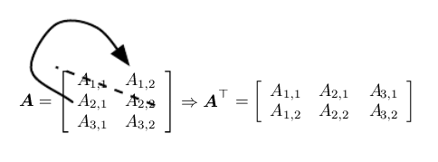
Transpose

An important operation on matrices.

Simply explained as mirroring a matrix across the main diagonal.

The six Vs

• Volume

• Variety

• Velocity

• Veracity

• Value

• Variability

Machine Learning

Step 1: Define a set of functions.

Step 2: Define the ‘goodness‘ of those functions.

Step 3: Pick the best function.

Supervised Learning

• Training data includes desired outputs, provided as pairs (x, y).

• Goal is to predict output ‘y’ from input ‘x’.

• Examples include: classification for discrete numbers, or regression for continuous numbers.

Unsupervised Learning

• Training data does not include desired outputs.

• Examples include Clustering and Dimensionality Reduction

Types of Learning

• Supervised

• Unsupervised

• Weakly or Semi-Supervised

• Reinforcement

Clustering

A process to find similarity groups in data.

Approaches include K-means, Fuzzy C-means, and Gaussiam Mixture Modelling.

K-means Clustering

• The number of clusters k is pre-set.

• Each data point is set to the nearest cluster centre or centroid.

• The process is iterative:

  • Each iteration assign each point to nearest centroid.

  • Move centroid to the centre of the group of points assigned to it. (Taking the average of the coordinates)

• Finish conditions:

  • Fixed number of iterations to begin with.

  • Repeat until “can not repeat” (the clusters are almost holding the same positions, so very small change in SSE)

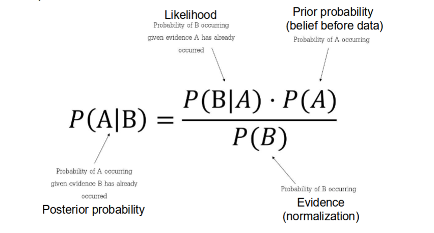
Conditional Probability

• Probability of an event or outcome occuring.

• Based on the occurence of a previous event or outcome.

• Calculated by multiplying the probability of the preceeding event by the updated probability of the succeeding, or conditional event.

Bayes’ Theorem

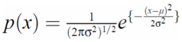
Guassian Distribution

Also known as a normal distribution.

Mu is the mean, sigma is the standard deviation.

A single function is usually not enough to model a histogram distribution, real world data is often multimodal.

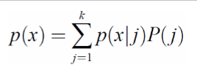
Guassian Mixture Modelling

• Each component (cluster) in the Guassian mixture has it’s own Guassian distribution assigned finally.

• Every cluster has it own size ( mu, sigma) or correlation (Sigma) with others.

• Compute the probability of each data sample that belongs to each cluster (by computing probability p(j | x)).

• Each cluster is approximately modelled by different updating Guassian distributions - an iterative process.

• Step 1:

  • Initialisation - Start from an initial guess of the parameters usually using K-means.

• Step 2:

  • Learning GMM Parameters: Posterioir probability - Compute posterior probabilty for each data point.

• Step 3: Learning GMM Parameters: Updating parameters

• Step 4: Repeat - Repeat 2 and 3 until convergence.

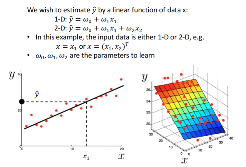
Linear Regression

How to avoid over-fitting?

1. Reduce model complexity

2. Early stopping

3. Increase sample number

4. Regularisation

5. For DL, use Transformation layer

Least Mean Squares

An adaptive optimisation algorithm used to find the best parameters (weights) that minimise the MSE or SSE between predicted and actual values.

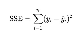
Sum Squared Error

Measure the difference between a model’s predictions and the real data by summing the squares of the differences between the observed and predicted values.

Where n is the number of observations, y_i is the value of the ith observation and y-hat_i is the predicted value for the ith data point.

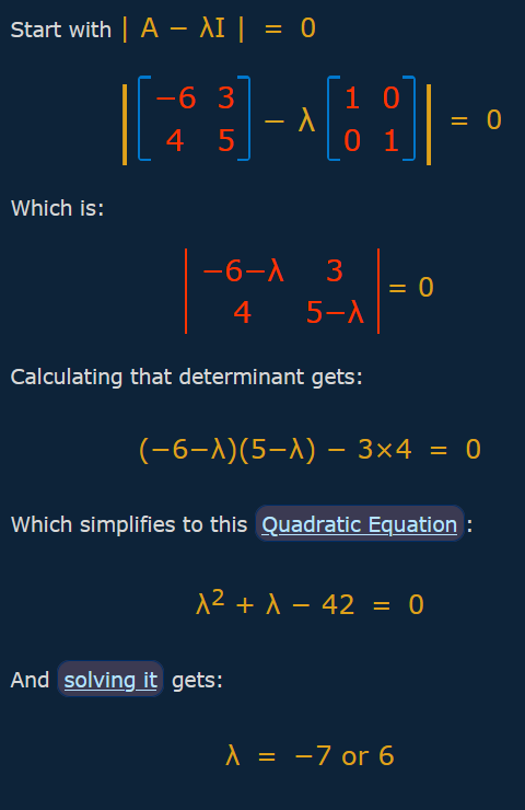
Eigenvalue

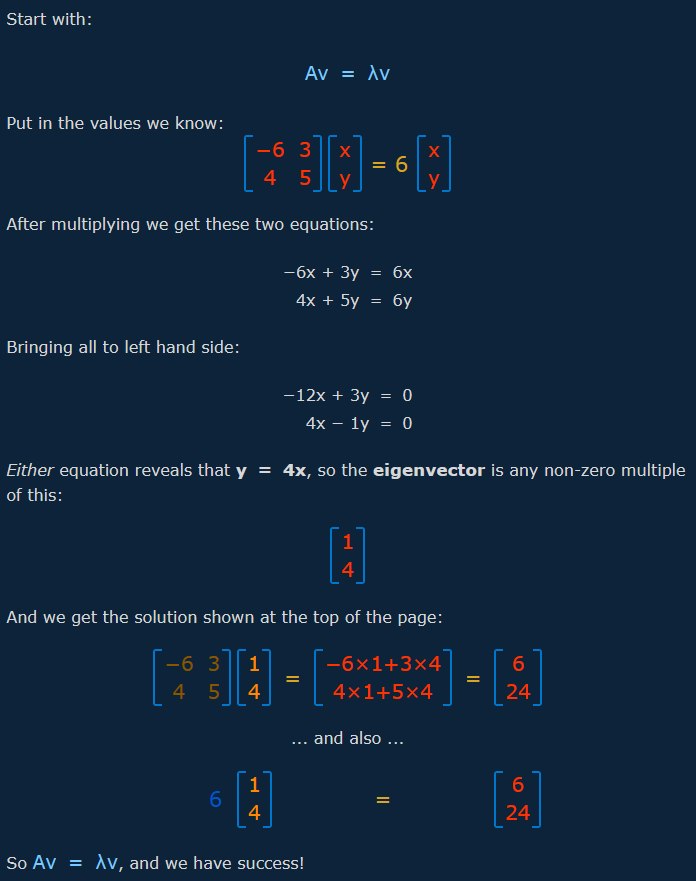
Eigenvector

Covariance

• Essentially multiply the rows of the two columns together and add them.

• cov(f1, f2) = first elem of f1 x first of f2 + second of f1 x second of f2….

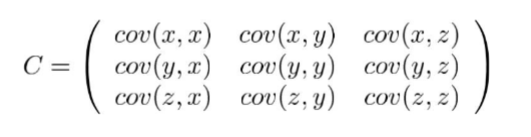
Covariance Matrix

• Example for 3-dimensional data.

• Is symmetrical about the main diagonal.

• Along the main diagonal, are the variance values.

• Axis- aligned spread is captured by the variance values, e.g. top left is low then low spread in x.

• Diagonal spread is captured by variance, positive meaning x increases as y does, negative, is opposite.

Principle Component Analysis

1. Standardise the dataset.

2. Calculate the covariance matrix.

3. Calculate the eigenvalues and eigenvectors for the covariance matrix.

4. Sort the eigenvalues and their corresponding eigenvectors.

5. Pick the top k eigenvalues and form a matrix of their eigenvectors.

6. Transform the original matrix by multiplying it by the matrix of eigenvectors.

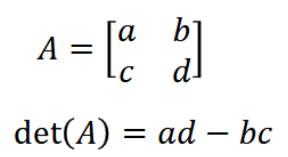
Determinent

• A single number that summarises the key properties of a square matrix.

• Usually used to measure how a matrix scales space.

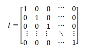
Identity Matrix

For an n x n matrix, it looks like this:

It has 1s on the main diagonal, and 0 everywhere else.

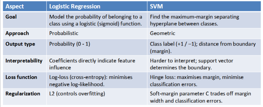
SVM

• Finds the optimal linear boundary (hyperplane) to divide data (binary classification).

• It aims for the maximum possible margin while minimising classification errors.

• If the data is not linearly seperable, use kernal functions, the “Kernal Trick“ converts non-linear data into a higher-dimensional feature space where it may be linearly separated.

Differences between logistic regression and SVMs

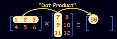
Matrix Multiplication

• To do this we need to find the dot product of rows and columns.

• The result will have the number of rows as the first matrix and number of columns as the second.

Components of CNN

• Convolutional Layers: These layers apply convolutional operations to input images using filters or kernels to detect features such as edges, textures and more complex patterns. Convolutional operations help preserve the spatial relationships between pixels.

• Pooling Layers: They downsample the spatial dimensions of the input, reducing the computational complexity and the number of parameters in the network. Max pooling is a common pooling operation where we select a maximum value from a group of neighboring pixels.

• Activation Functions: They introduce non-linearity to the model by allowing it to learn more complex relationships in the data.

• Fully Connected Layers: These layers are responsible for making predictions based on the high-level features learned by the previous layers. They connect every neuron in one layer to every neuron in the next layer. A fully connected network alone might not do well at image classification without other layers extracting high level features for it.

Softmax

Converts the raw output scores or logits generated by the last layer of a neural network into a probability distribution. The function exponentiates each logit and then normalizes the results, ensuring that the output values fall between 0 and 1 and sum up to 1. This makes the output interpretable as class probabilities.

This is particularly suited for multi-class classification problems, as it provides a clear and normalized probability distribution across all possible classes.

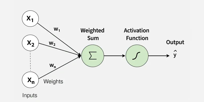
Perceptron

1. Inputs (x1,x2,...,xn)(x1​,x2​,...,xn​)

These are the features or measurable attributes of a data points that are used to make a decision. Each input provides a signal that contributes to the final output.

• Inputs themselves have no inherent influence unless multiplied by weights.

2. Weights (w1,w2,...,wn)(w1​,w2​,...,wn​)

Weights determine how strongly each input contributes to the prediction. A larger weight means the corresponding input has a higher impact.

• Weights are learned during training, adjusting based on errors.

• They act like importance scores for each feature.