meteorology

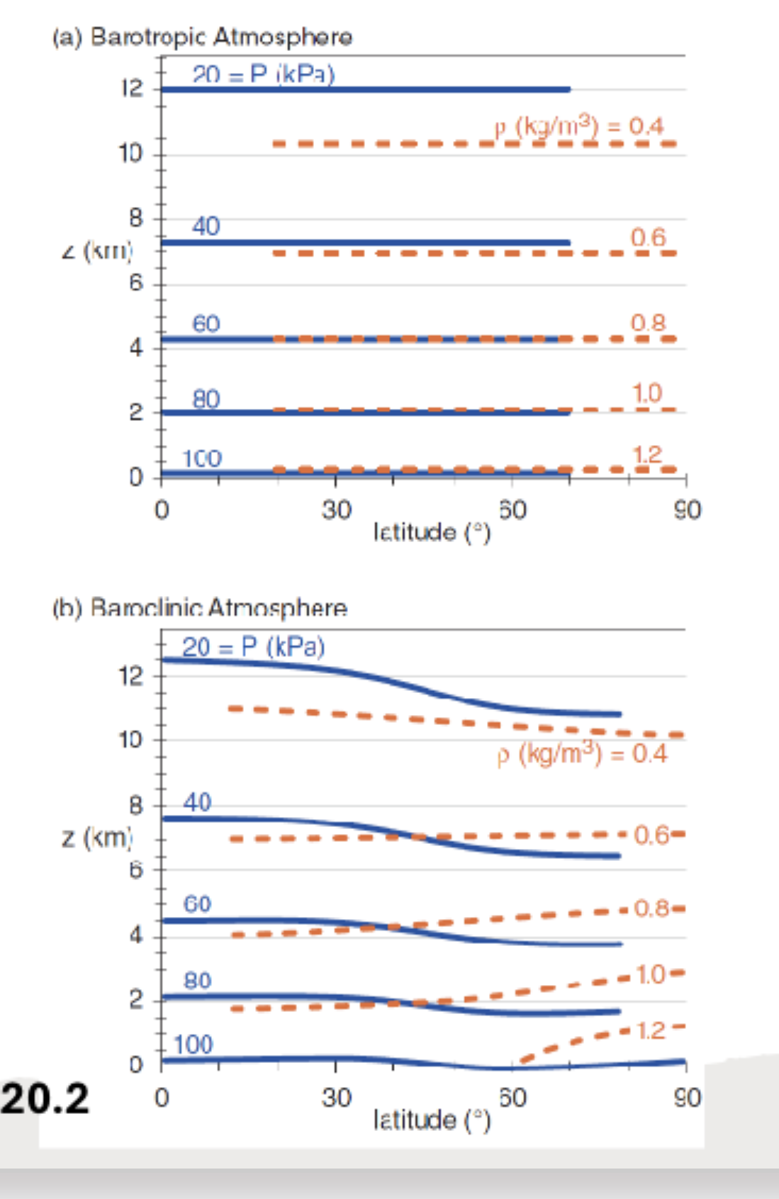
Figure 20.2 displaying the barotropic atmosphere and the baroclinic atmosphere pressure, height, and latitude

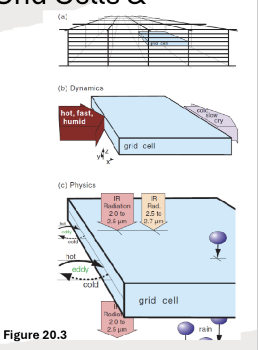
20.3 A forecast domain divided into 3-D grid cells (a,b,c)

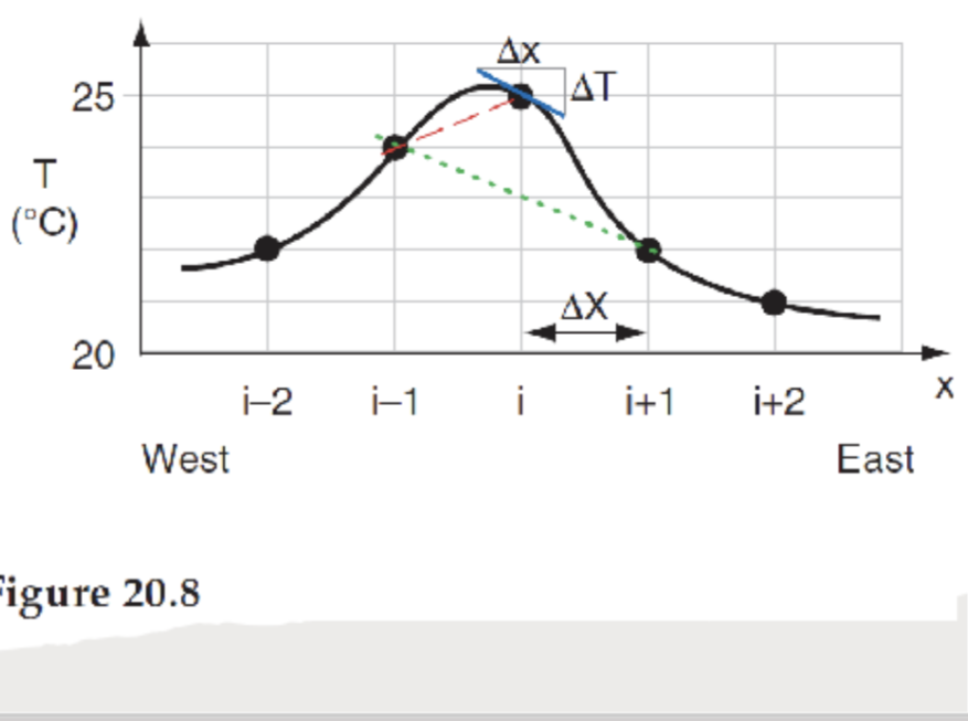
20.8 Finite difference methods of estimating the slope at grid point i

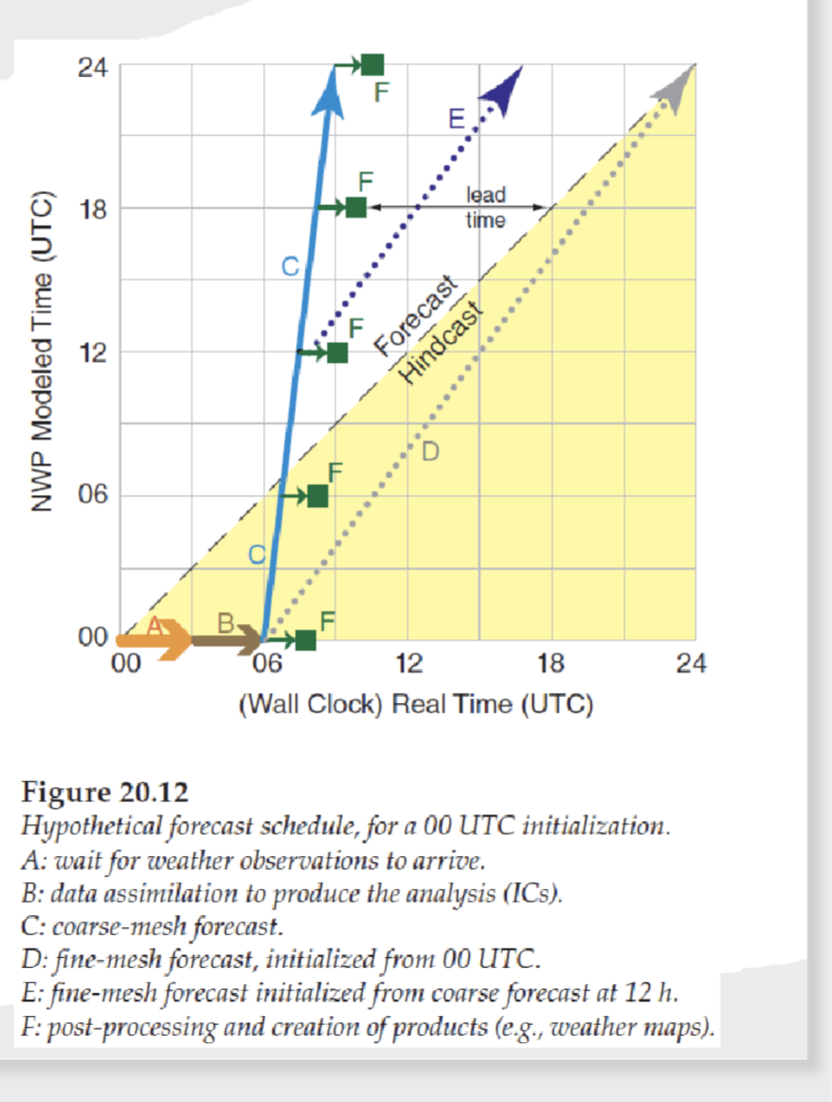
20.12 Weather forecasting schedule, showing observation delay and data assimilation delay

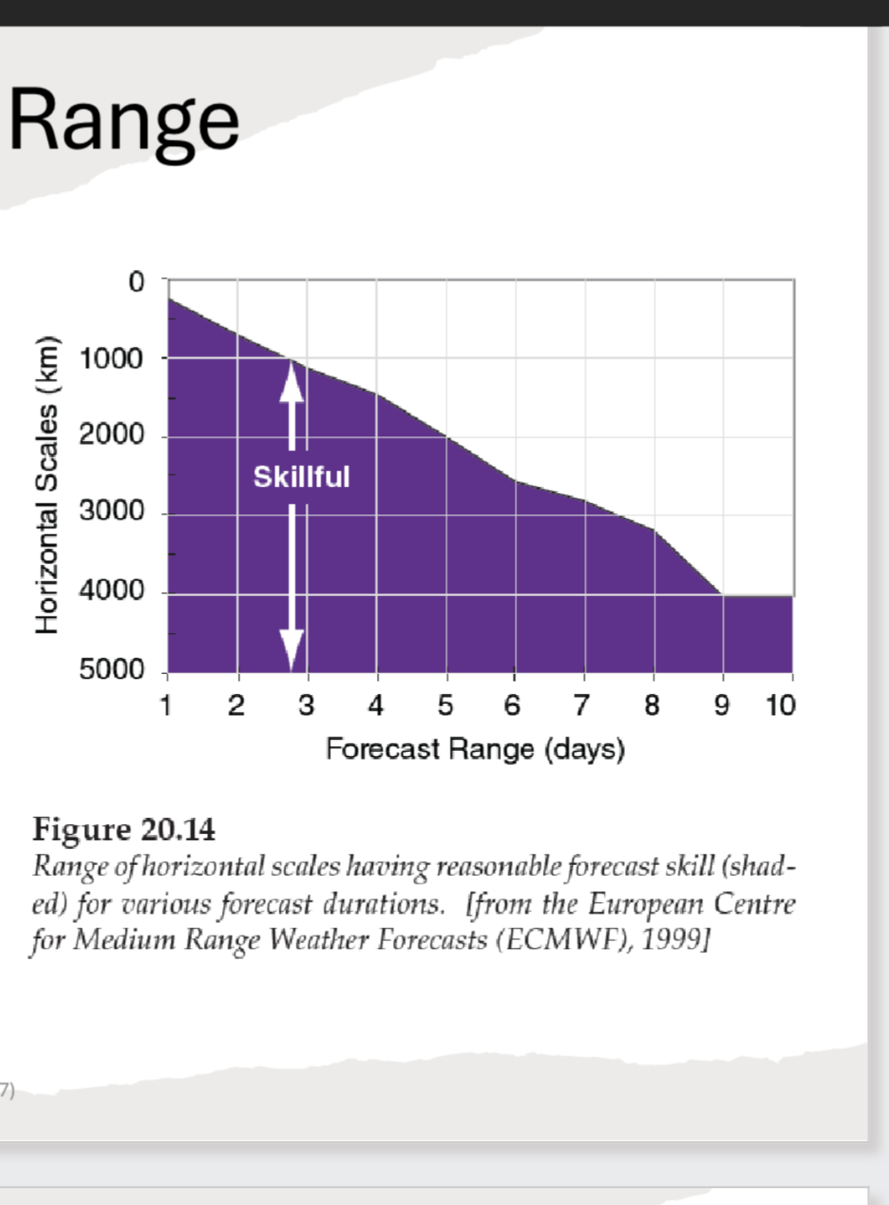
20.14 range of horizontal scales having reasonable forecast skill

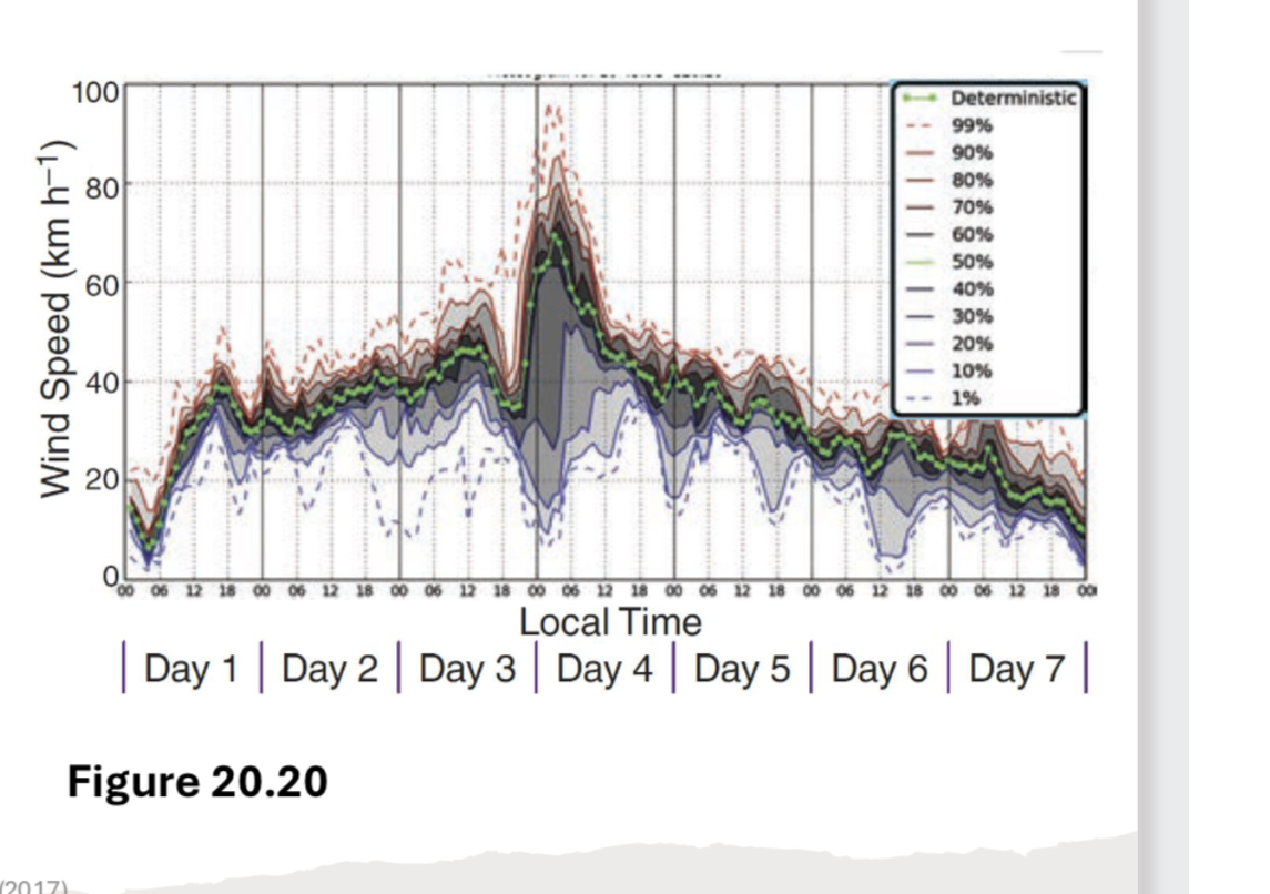
20.20 deterministic forecast showing predicted daily outcome

enables us to bound uncertainty

20.22 NWP model forecast displaying forecast day and anomaly correlation

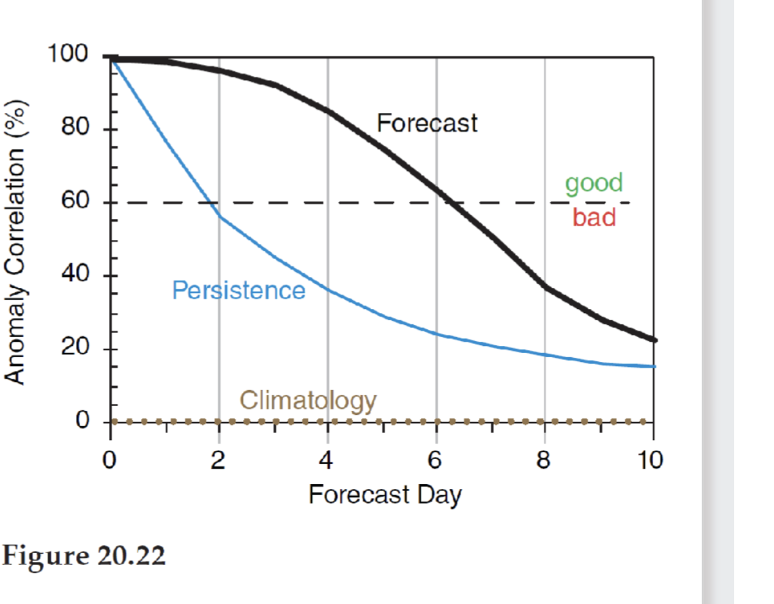
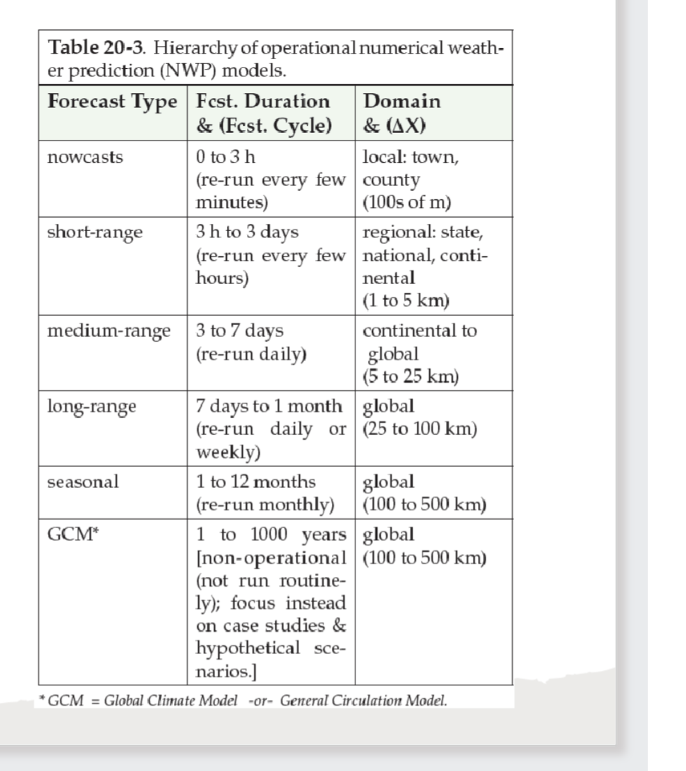
Table 20-3 Hierarchy of operational numerical weather prediction models

know at least three

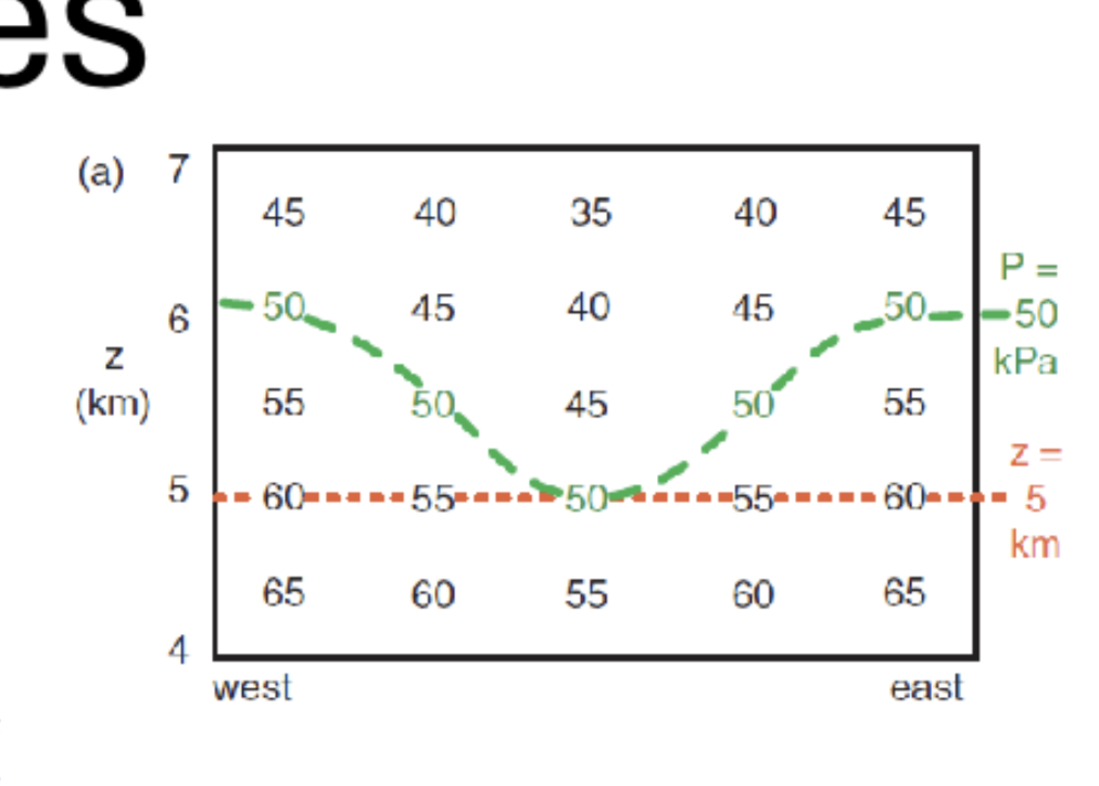
10.2a pressures differing at locations, chart of pressures and variable line with height line

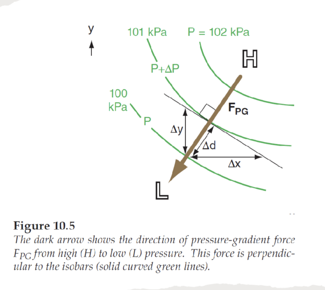
10,.5 horizontal pressure gradiant force perpendicular to isobars

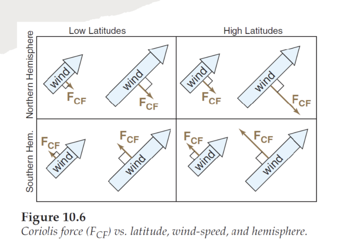
10.6 Coriolis force displayed at low lat, high latitude, comparing northern and southern hemisphere

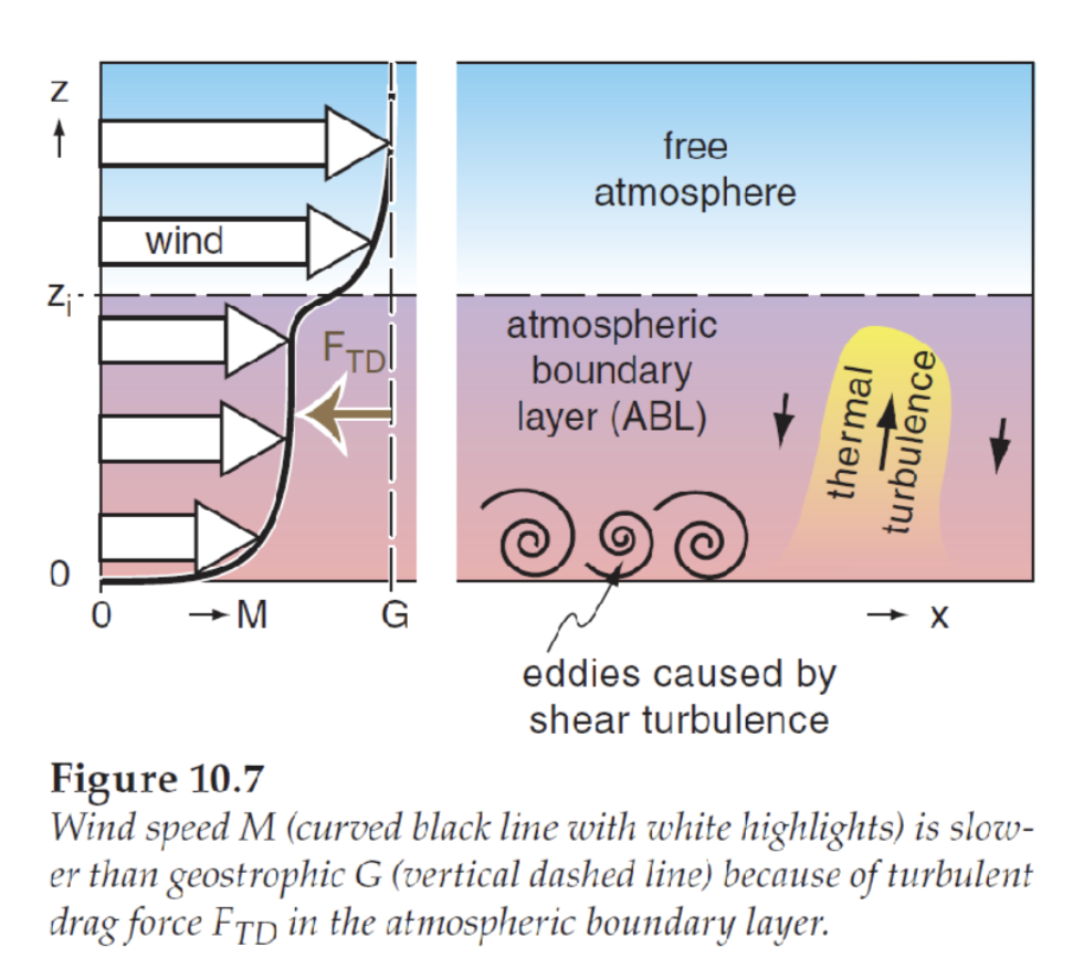
10.7 Turbulent drag force in the atmospheric boundary layer making wind speed slower than geostrophic G

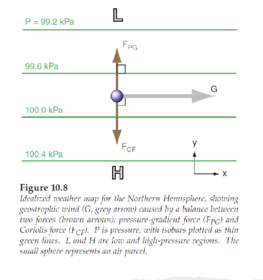
10.8 idealized weather map showing geostrophic winds caused by a balance between two forces: pressure gradient force and Coriolis force

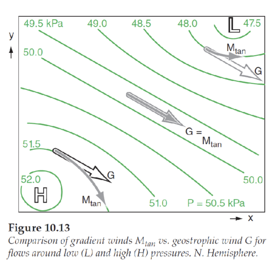
10.13 comparison of gradient winds vs geostrophic winds for flows around. low and high pressure in the northern hemisphere

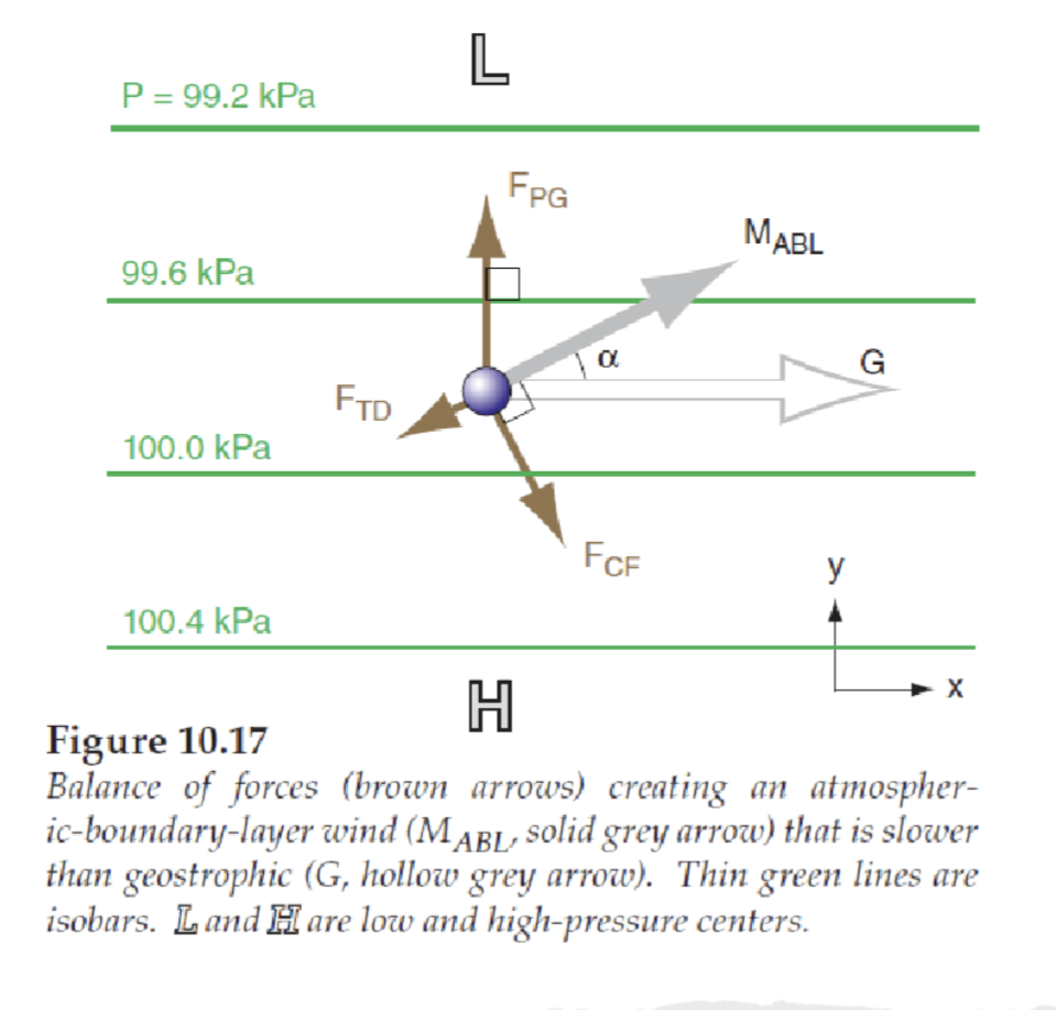
10.17 Balance of forces creating an atmospheric boundary layer wind that is slower than geostrophic winds

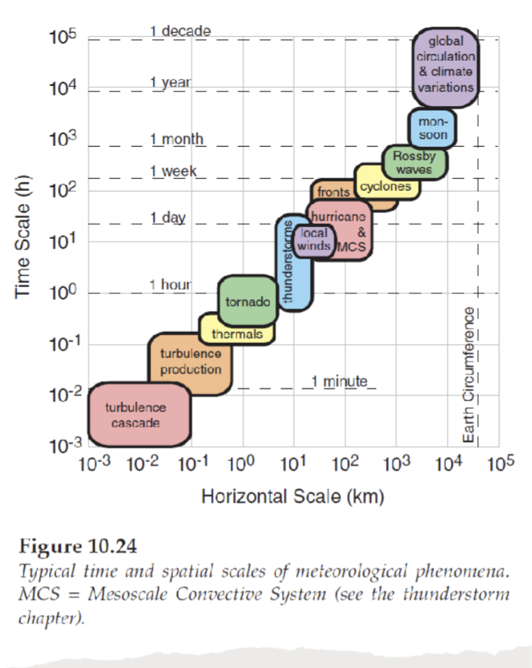
10.24 typical time and spatial scales of meteorological phenomena

10.27 volume conservation for an idealized cylindrical extratropical cyclone

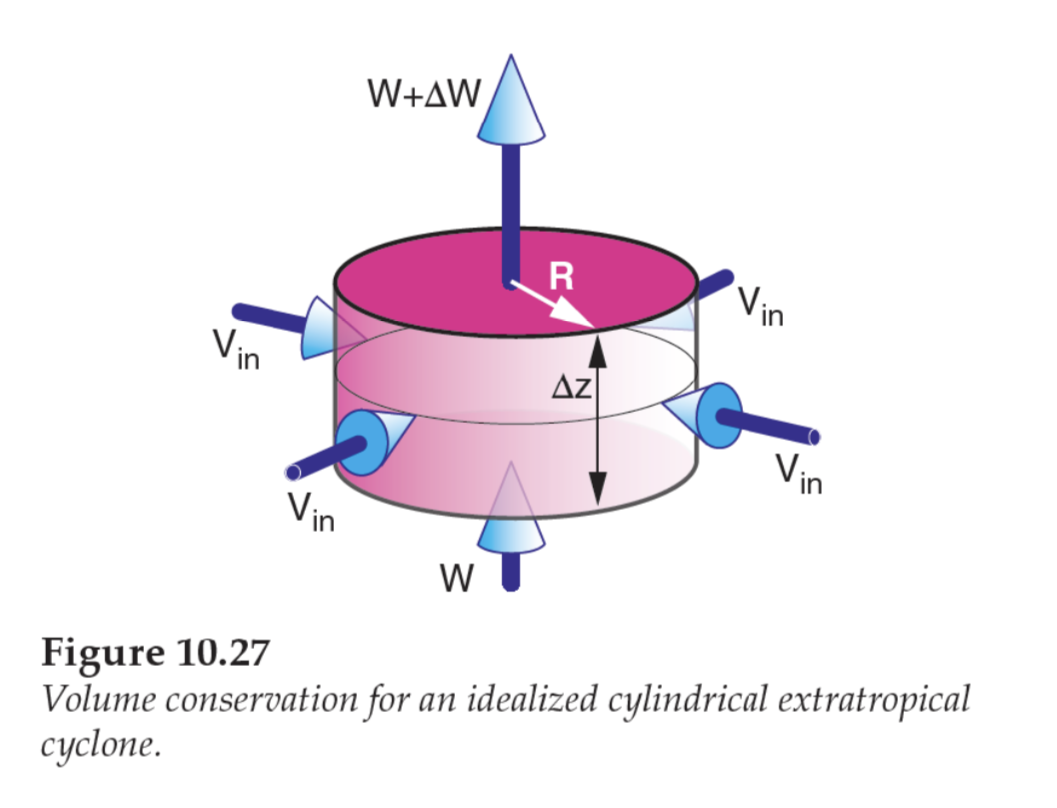
Table 10-3 summary of forces

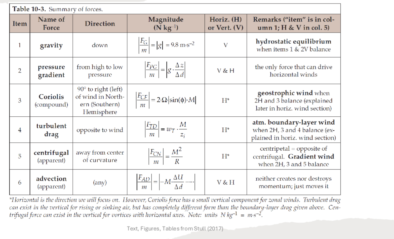
Table 10-5 summary of horizontal winds

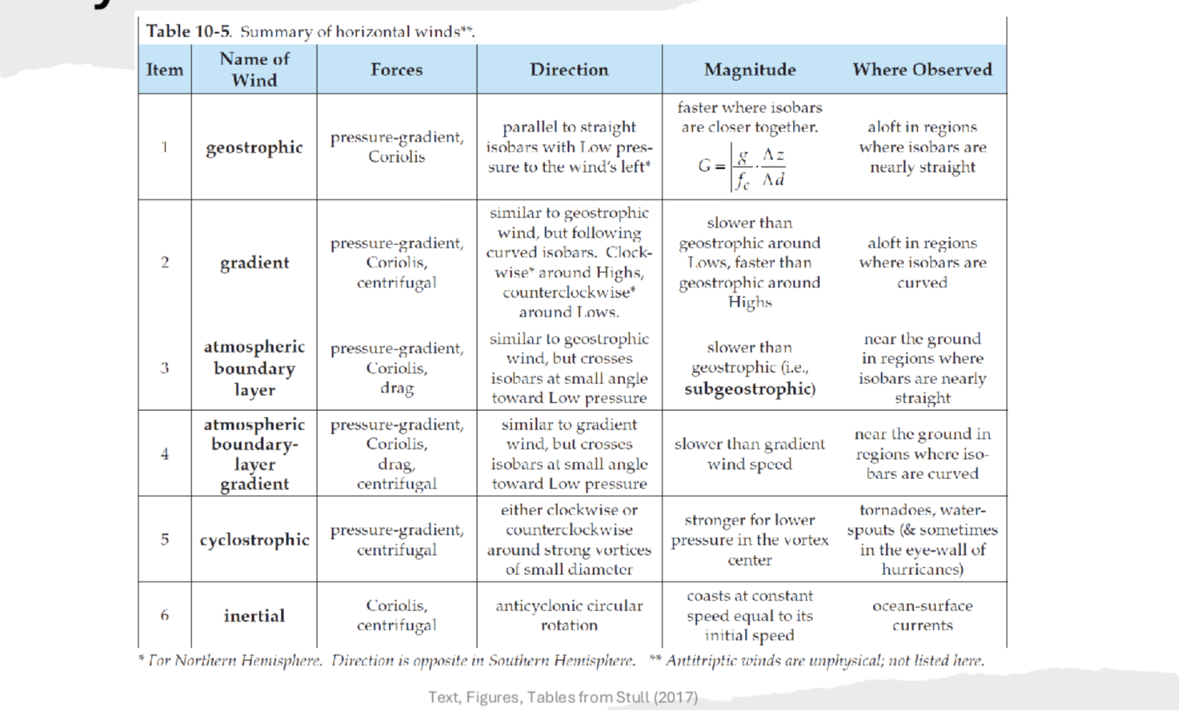
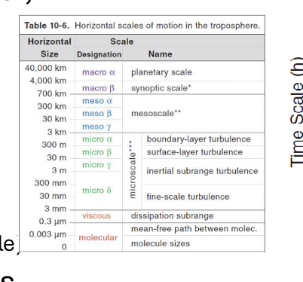
Table 10-6 horizontal scales of motion in the troposphere

4 ranges and names

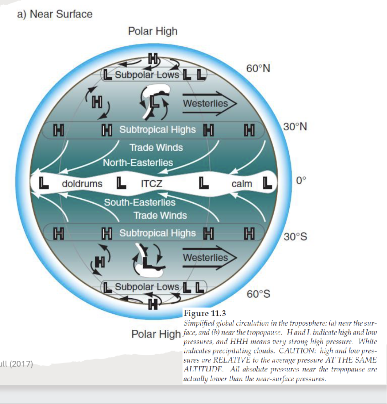
11.3a simplified global circulation in the troposphere near the surface

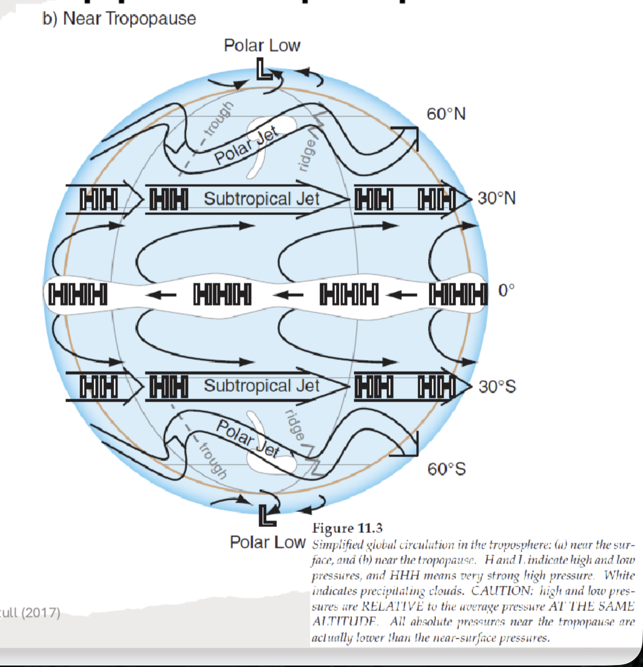
11.3b simplified global circulation near the tropopause

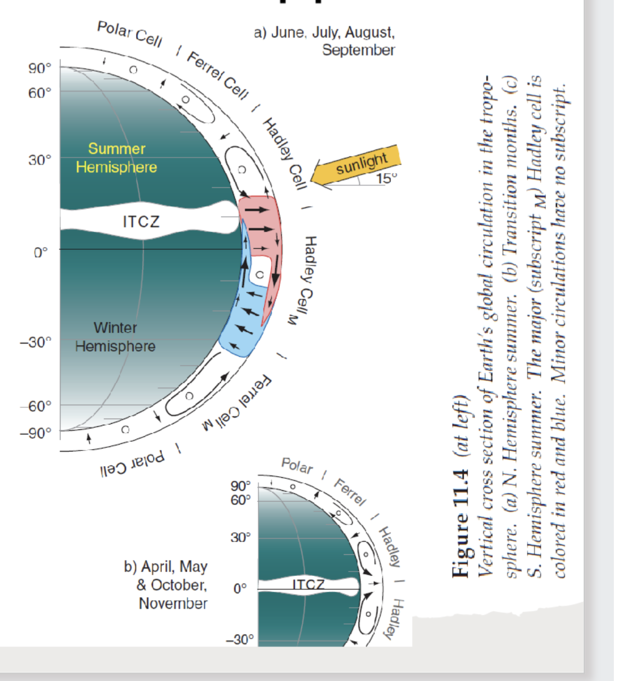
11.4 vertical cross section of earths global circulation in the troposphere

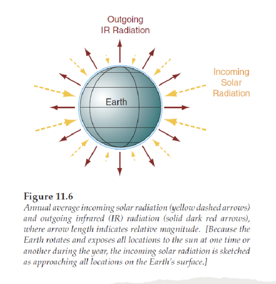
11.6 annual avg incoming solar radiation and outgoing infrared radiation where arrow length indicates magnitude

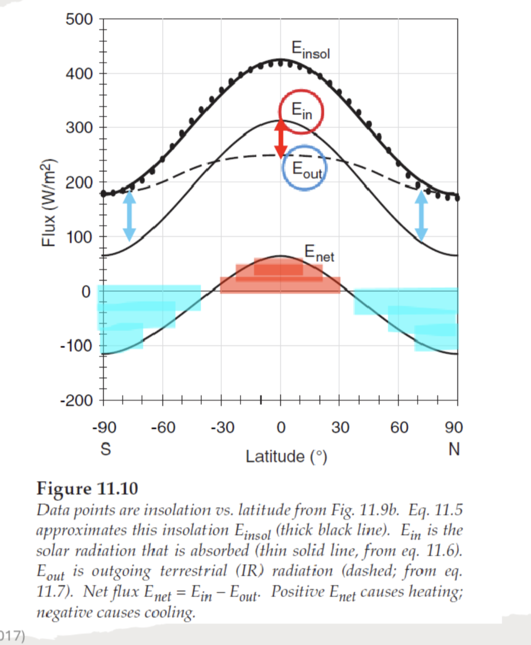
11.10 graph displaying outgoing terrestrial radiation in and out , insolation, and net flux

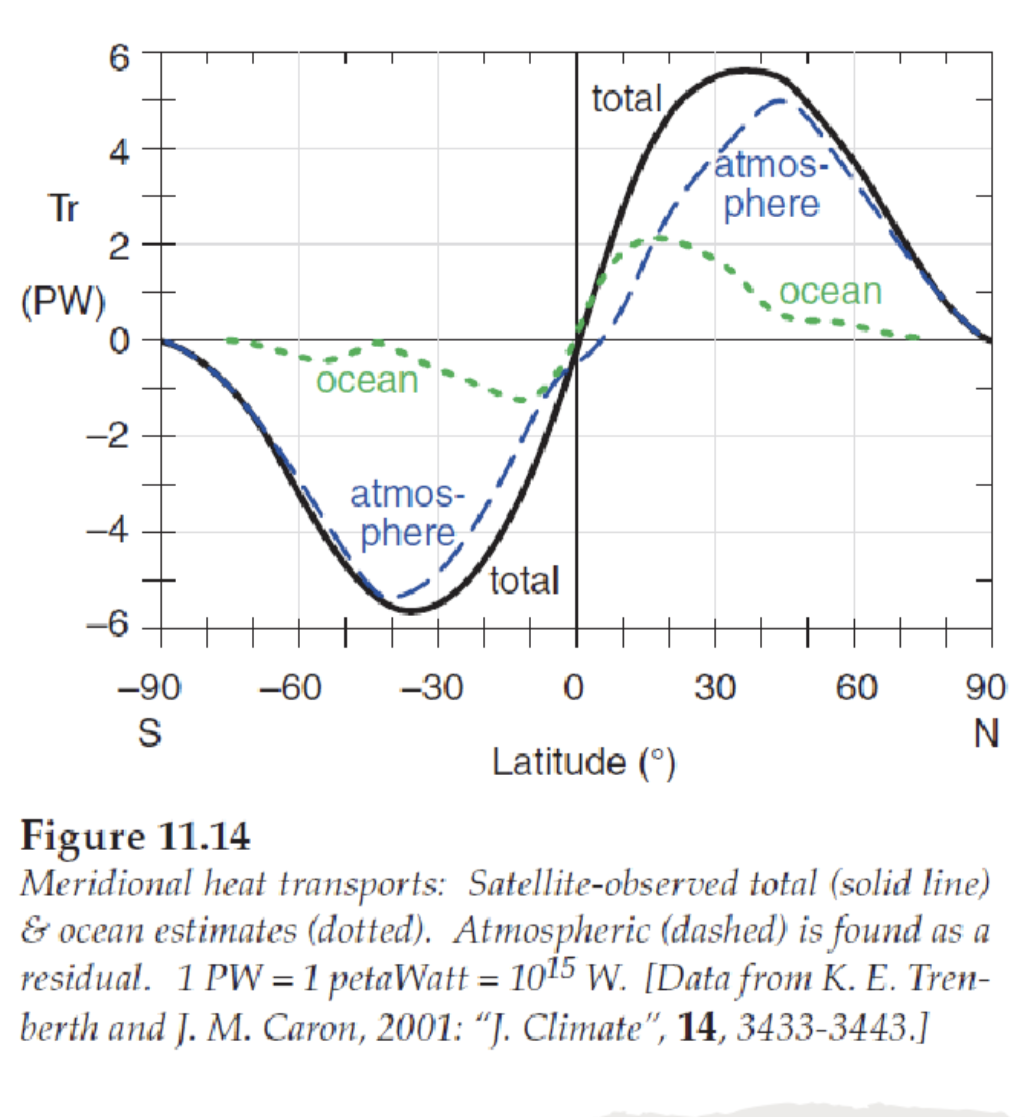
11.14 meridional heat transports: satellite observed total and ocean estimates. Atmospheric is found as a residual

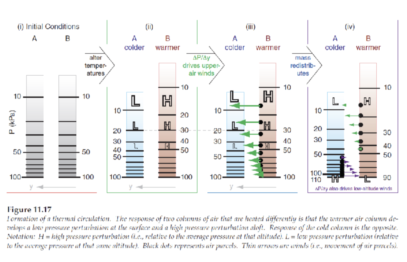
11.17 formation of thermal circulation. The response of two columns of hair that are heated differently

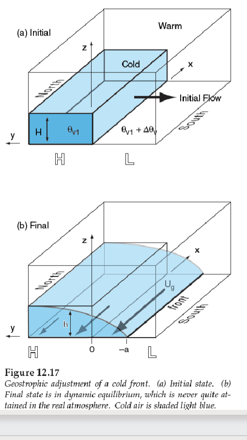
know initial state and final state

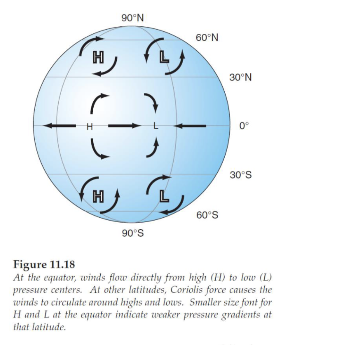
11.18 circulation mechanisms and geostrophic winds at the equator flowing directly from high to low pressure centers. at other latitudes the Coriolis force causes winds to circulate around highs and lows

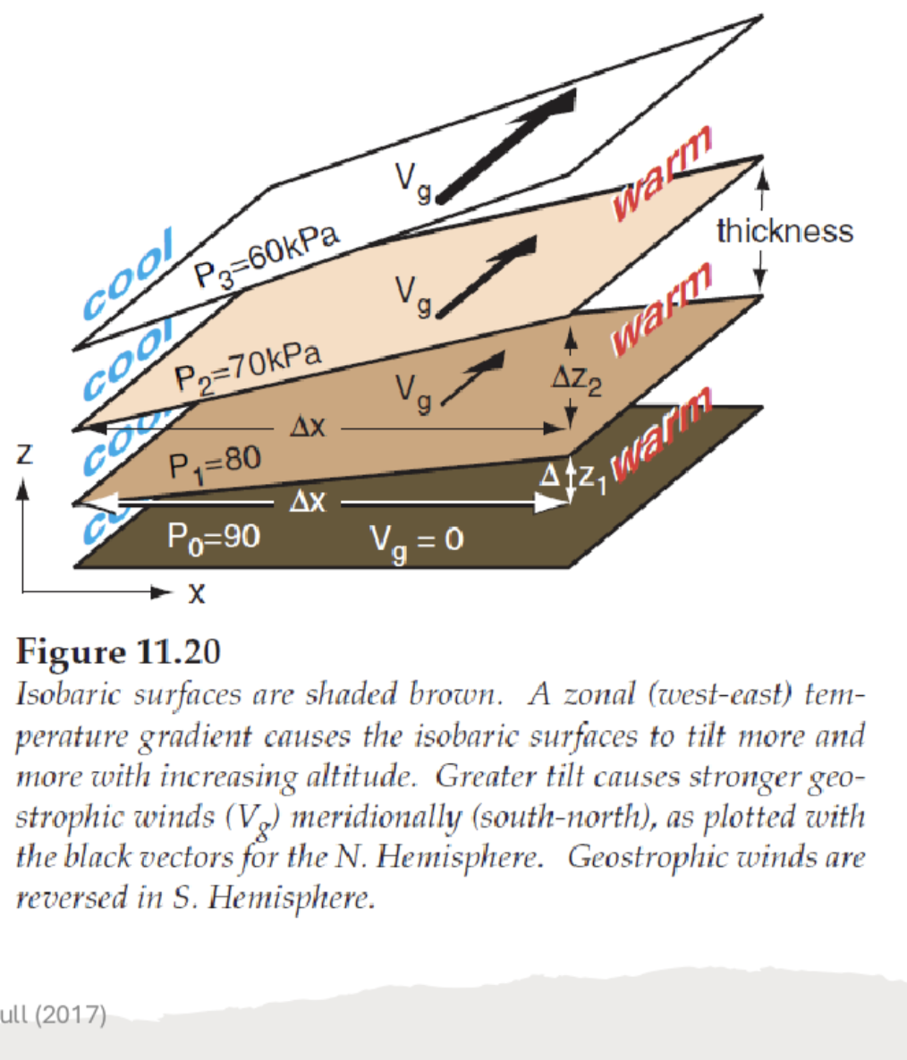
11.20 a zonal temperature gradient causes isobaric surfaces to tilt with increasing altitude. greater tilt causes greater geostrophic winds.

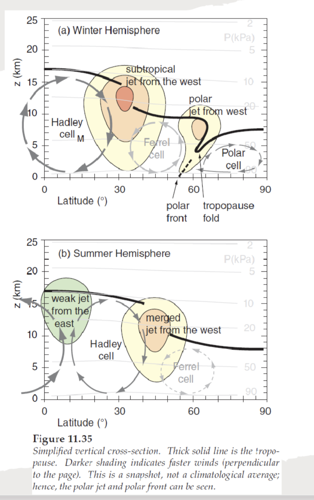
11.35 simplified vertical cross section displaying polar and subtropical jet streams in winter and summer hemisphere

freebie

c- continental m-maritime t-tropical p-polar

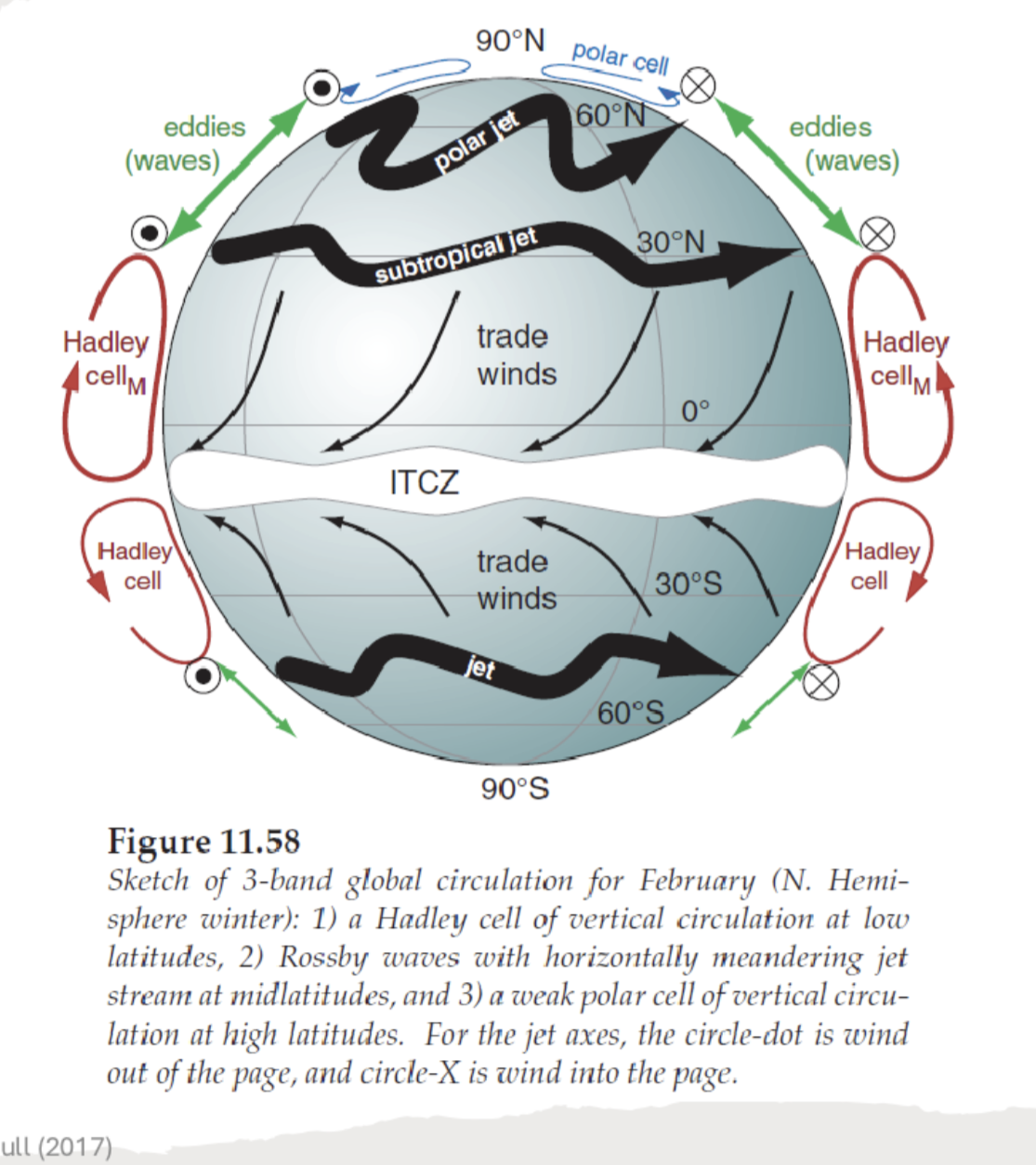
11.58 sketch of 3 band global circulation for February

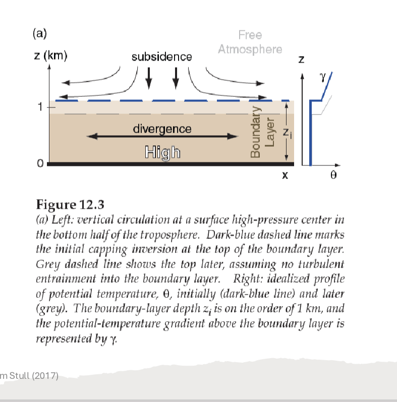
12.3 vertical circulation at surface high-pressure center in the bottom half of the troposphere

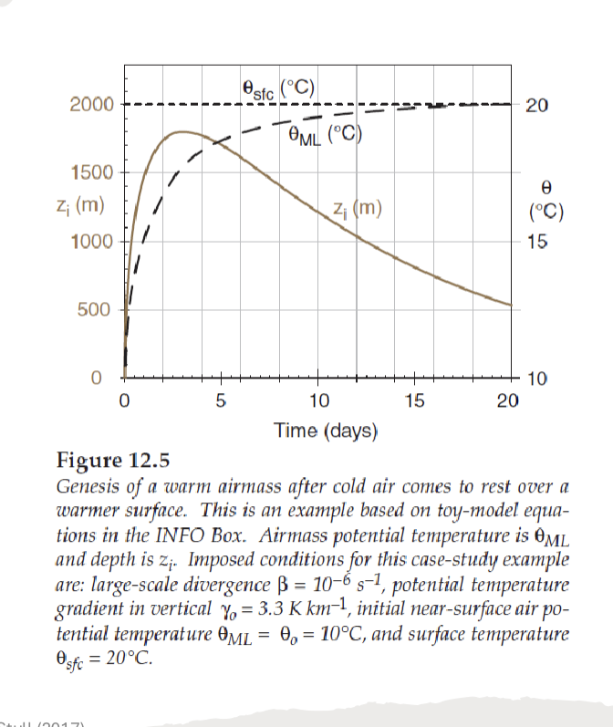
12.5 warm air mass genesis after cold air comes to rest over a warmer surface

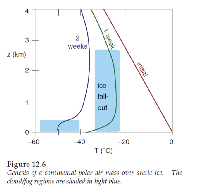
12.6 Genesis of a continental-polar air mass over arctic ice

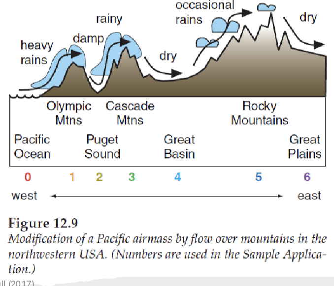
12.9 Modifications of a Pacific airmass by flow over mountains in the northwestern USA

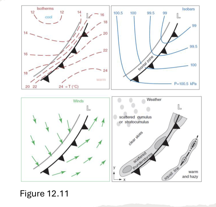
12.11 cold fronts displaying four graphs of isotherms, isobars, winds, and weather

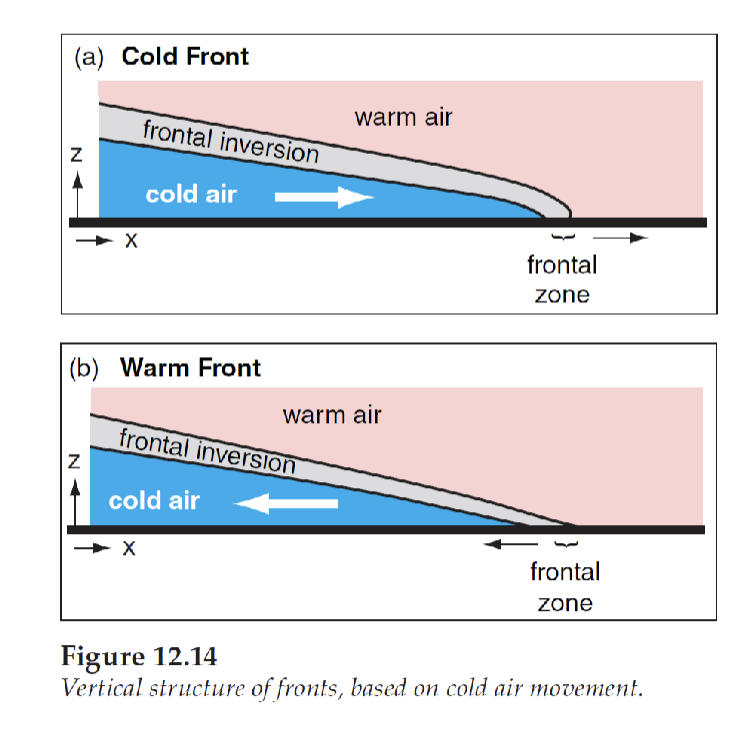
12.14 Vertical structure of fronts, based on cold air movement

12.17 Geostrophic adjustment of a cold from. (a) initial state. (b) final state is in dynamic equilibrium which is never quite attained in the real atmosphere

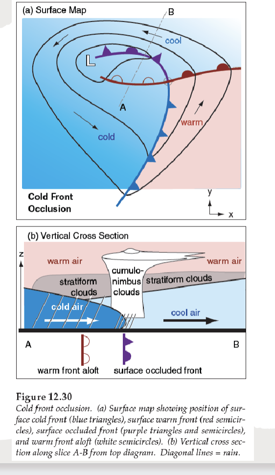
12.30 Cold front occlusion (a) surface map showing position of surface cold front, surface warm front, surface occluded front, and warm front aloft. (b) vertical cross section along slice A-B from top diagram

12.31 Warm front occlusion (a) surface map, symbols are to fig 12.30. (b) vertical cross section along slice C-D from top diagram

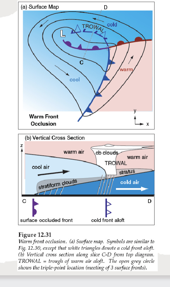
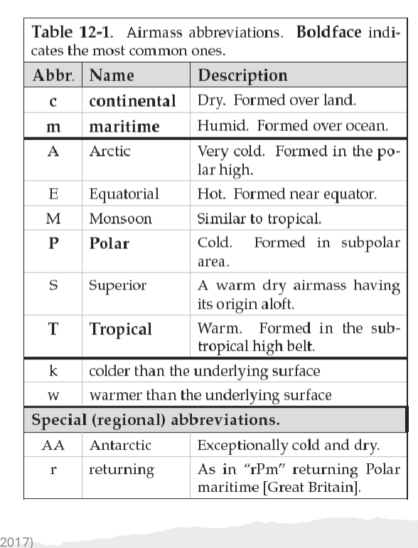
Table 12.1 Airmass abbreviations

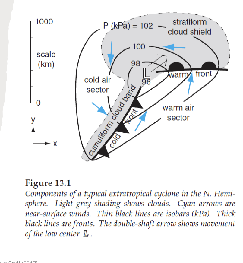
13.1 Components of a typical extratropical cyclone in the northern hem.

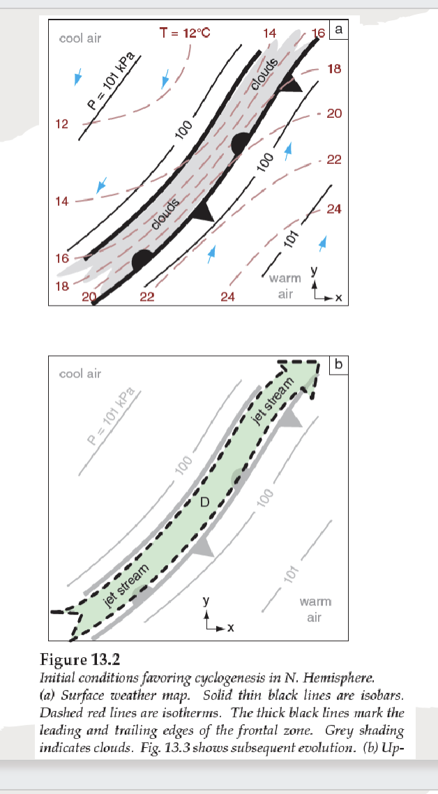
13.2 Initial conditions favoring cyclogenesis in northern hemisphere (a) surface weather map (b) upper air jet stream

(b)

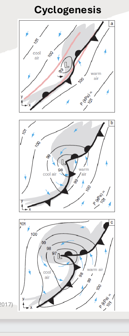
13.3a-c the three stages of cyclogenesis

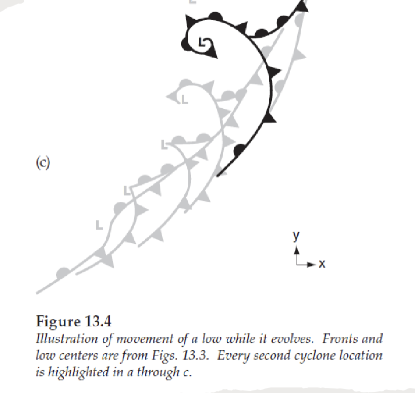
13.4b illustration of movement of a low while it evolves

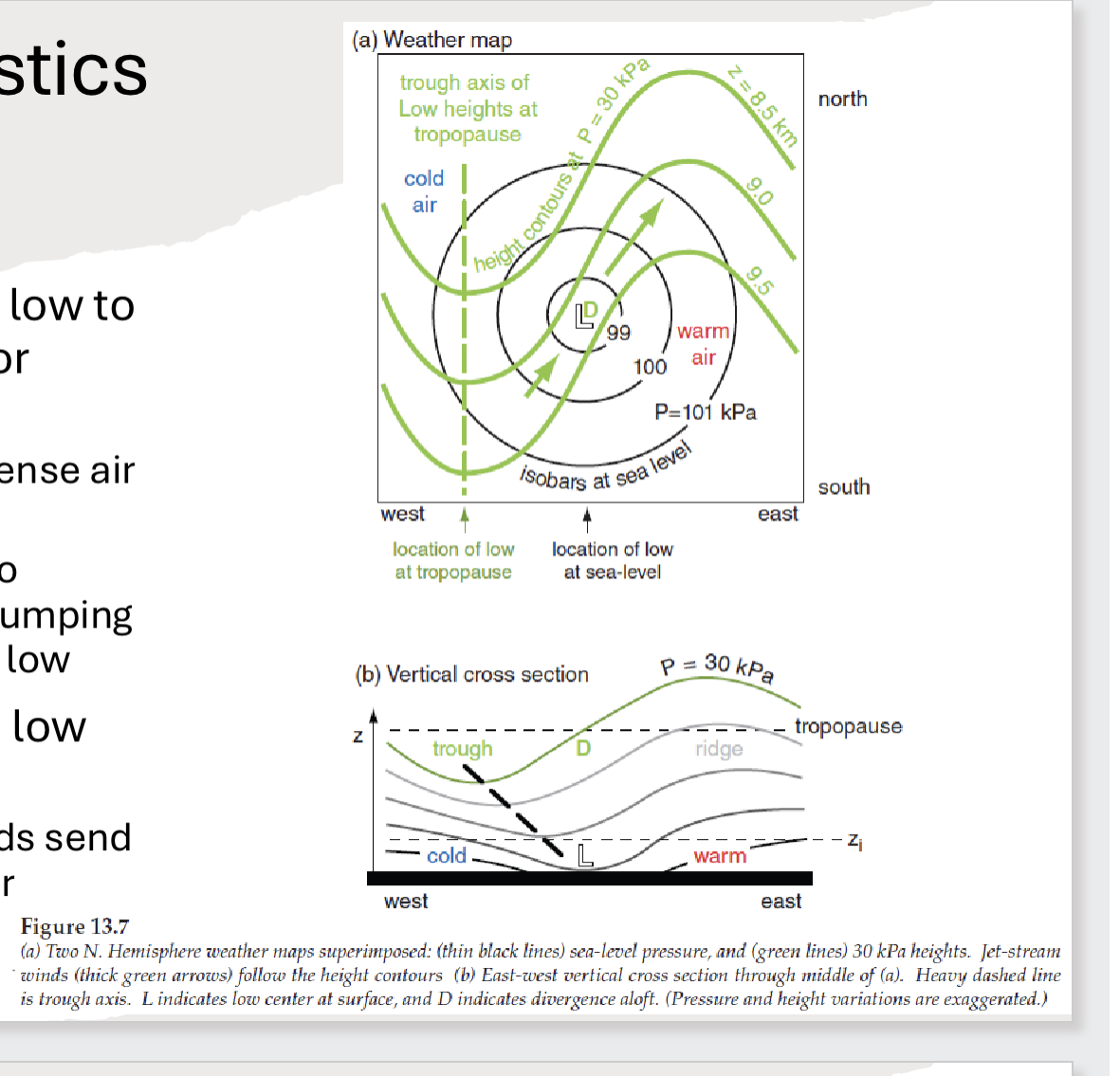
13.7 two n. hem. weather maps superimposed displaying vertical tilting from surface low to upper level trough allowing cyclogenesis, and vertical stacking filling the low leading to cyclolysis

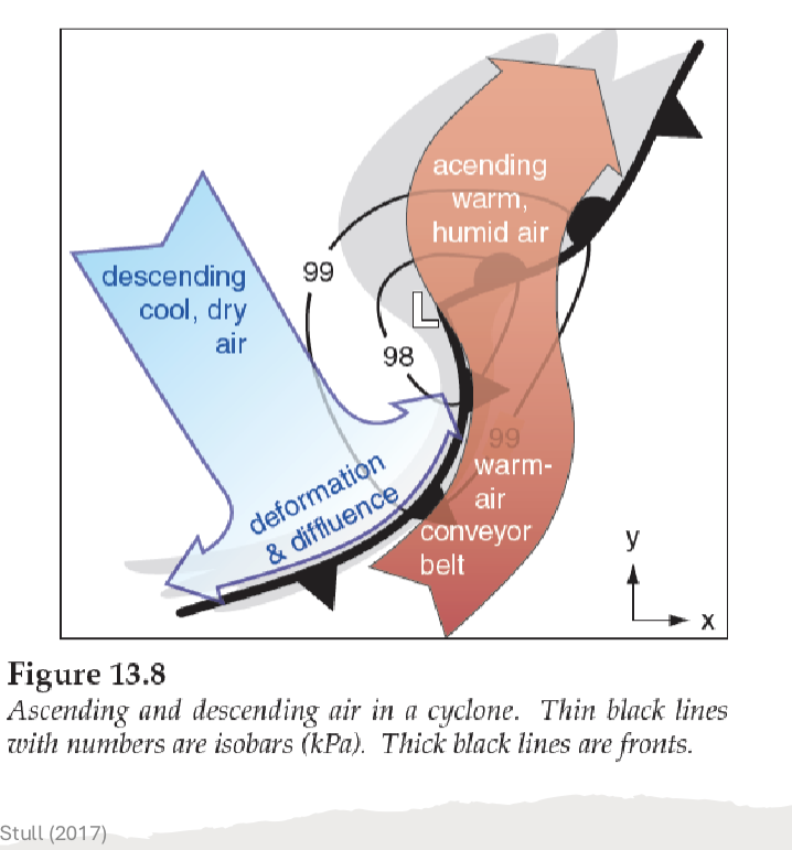
13.8 ascending and descending air in a cyclone

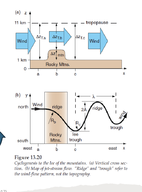
13.20 Cyclogenesis to the ice of the mountains. (a) vertical cross section (b) map of jet stream flow.

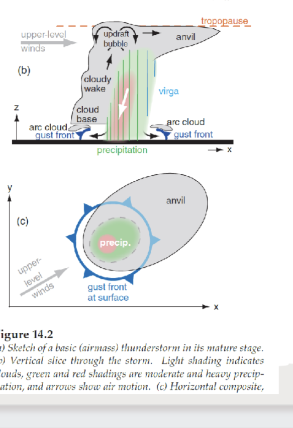
14.2 vertical slice through mature thunderstorm (c ) horizontal composite

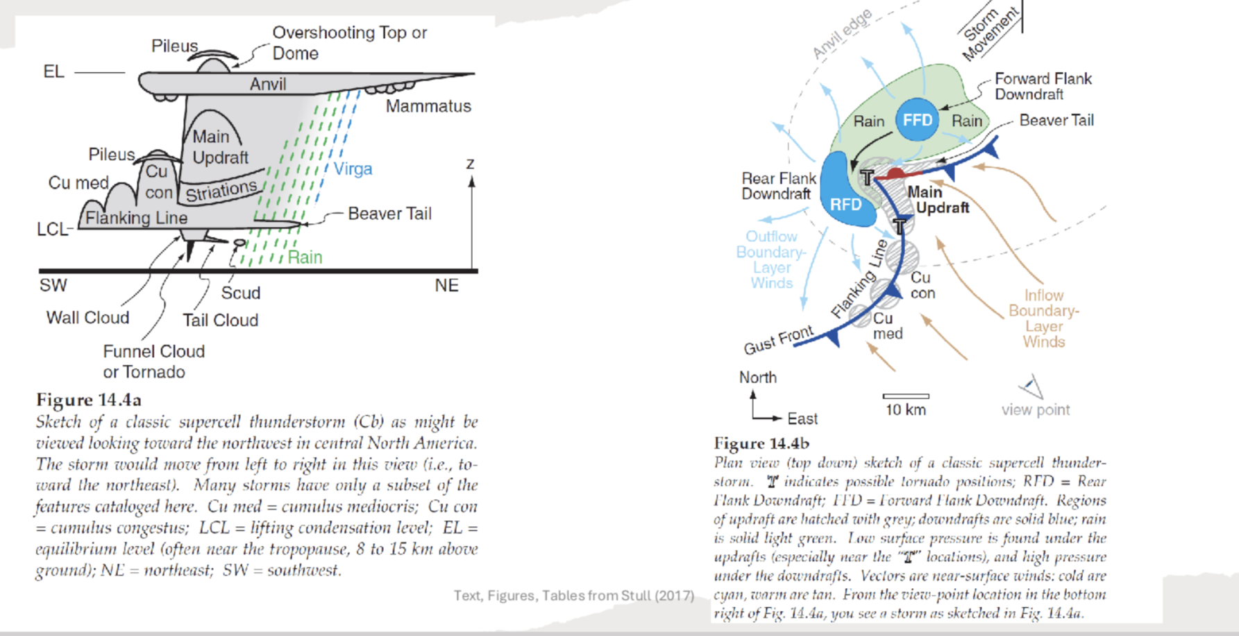
14.4 a-b sketch of classic supercell thunderstorm moving left to right. top down view sketch of a classic supercell showing possible tornado positions

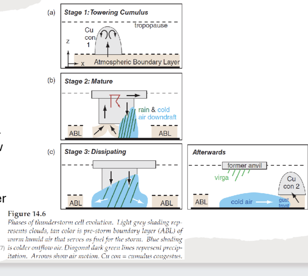
14.6 phases of thunderstorm cell evolution- towering cumulus, mature, dissipating, afterwards

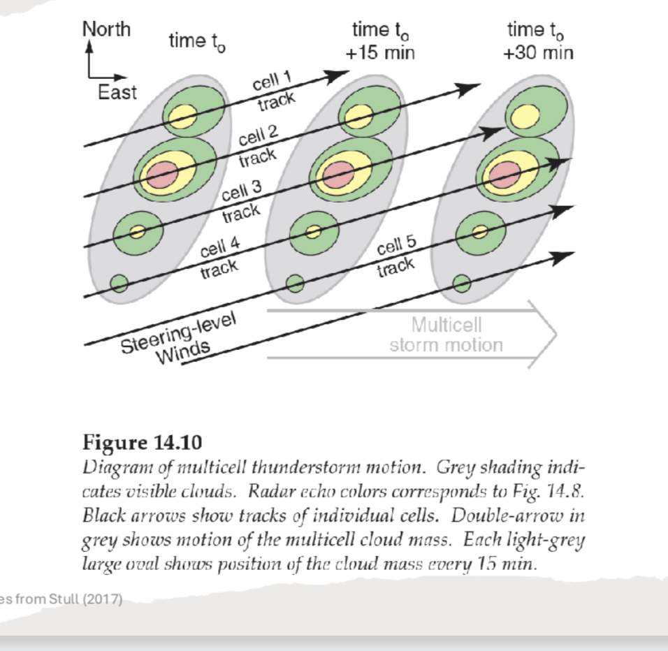
14.10 diagram of multicellular thunderstorm motion at 15 min increments

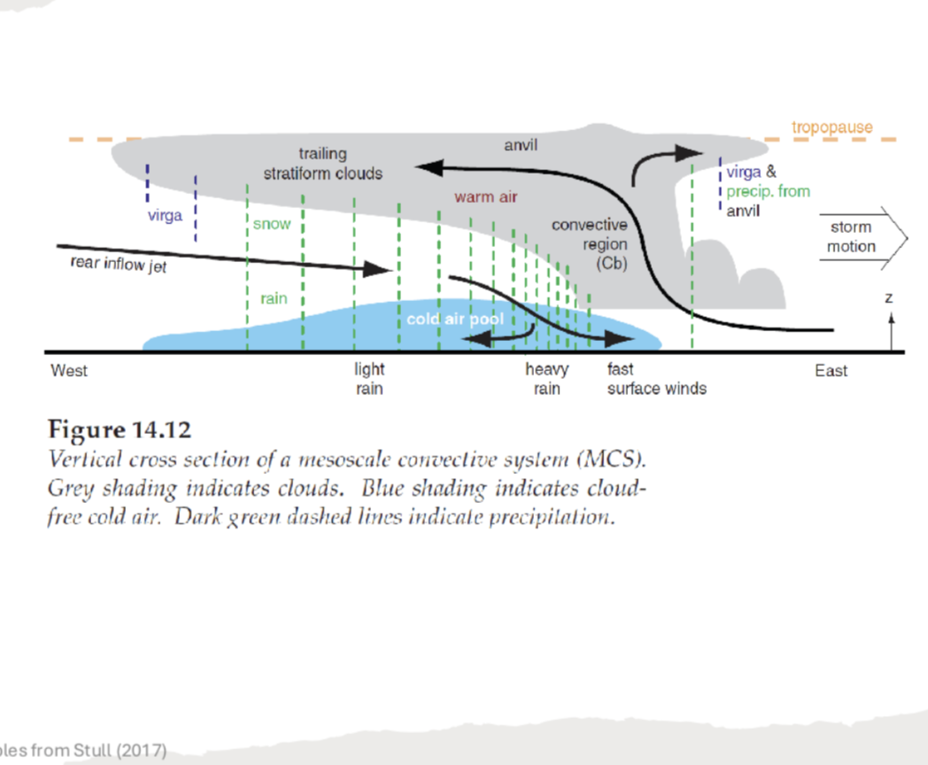
14.12 vertical cross section of a mesoscale convective system

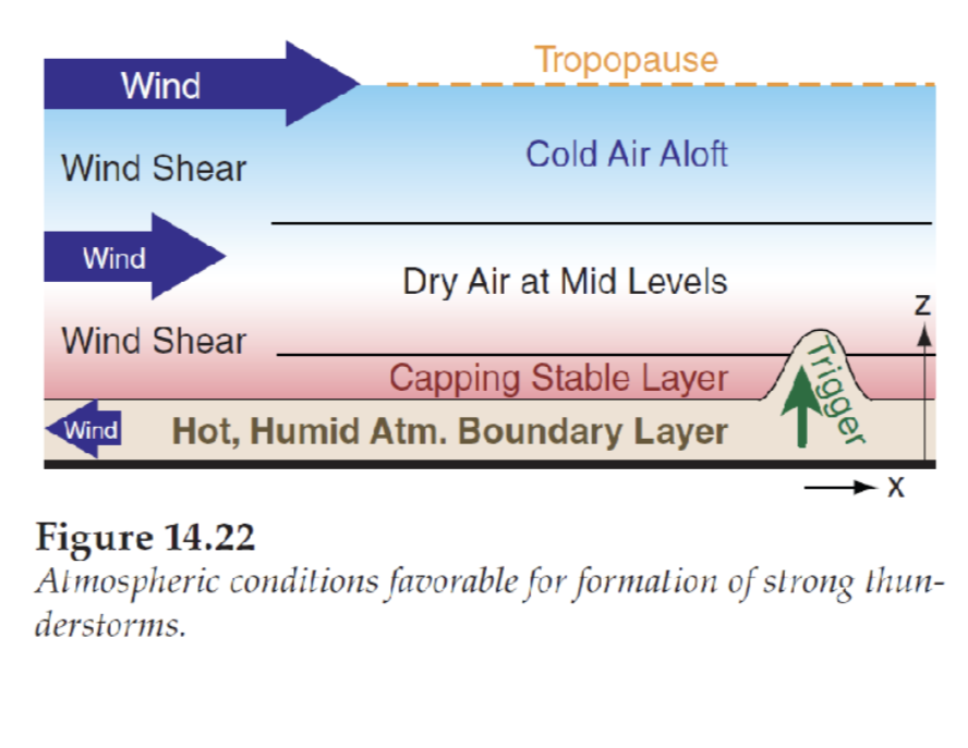
14.22 atmospheric conditions favorable for formation of strong thunderstorms

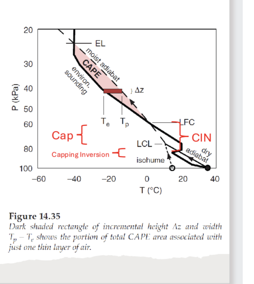
14.35 sketched rectangle of incremental height (change in z) and width Tp-Te shows the portion of total CAOE area associated with just one thin layer of air

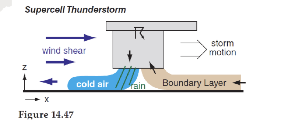
14.47 sketch of supercell thunderstorm with changing wind shear

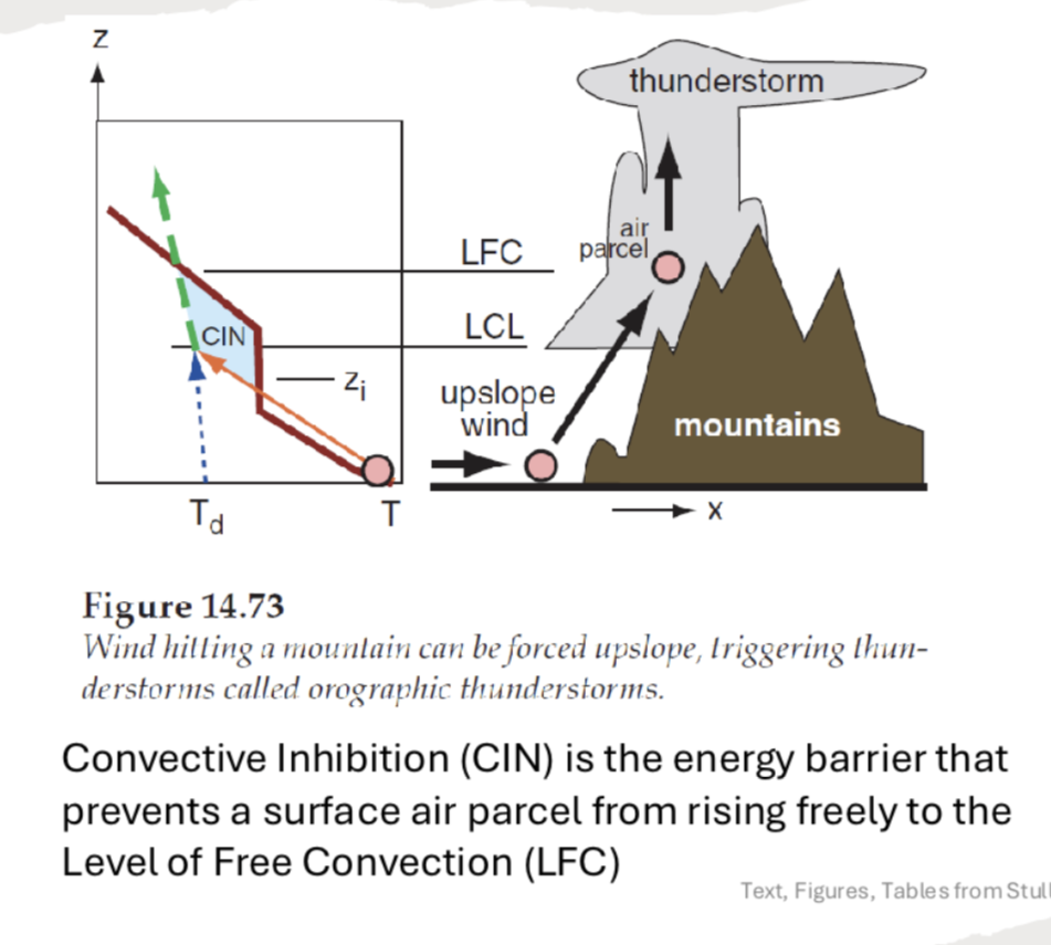
14.73 wind hitting a mountain can be forced upslope, triggering thunderstorms called orographic thunderstorms

14.76 (a-b) simplification of daily cycle of upward net radiation, which combines solar heating during the day and infrared cooling day and night, for summer over land

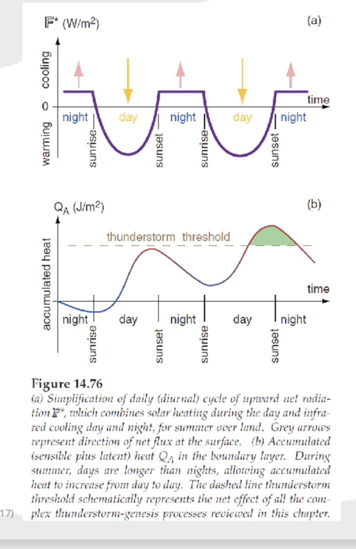
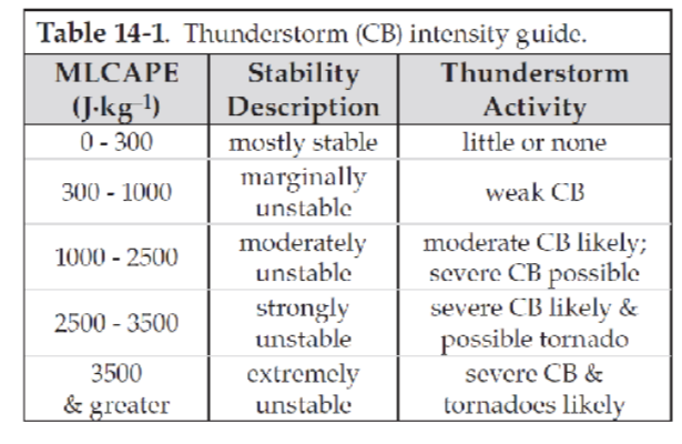
table 14-1 thunderstorm intensity guide