I PRAY to STATS – Core Vocabulary

Key statistical vocabulary extracted from the 'I PRAY to STATS' lecture notes, covering basic descriptive statistics, sampling methods, experimental design, common fallacies, graphical displays, regression, probability distributions, confidence intervals, hypothesis testing, and useful combinatorial principles.

Mean (Arithmetic)

Sum of all measurements divided by the number of observations; symbol μ for a population and x̄ for a sample.

Median

The middle value that splits an ordered dataset into two equal halves.

Mode

The most frequently occurring value in a dataset.

Interquartile Range (IQR)

Difference between the third quartile (Q3) and the first quartile (Q1); measures spread of the middle 50 %. IQR = 3 - Q1

Range

Largest value minus smallest value in a dataset; a crude measure of variability.

Standard Deviation (σ or s)

A measure of the amount of variation a variable has about its mean. σ for a population. s for a sample. For a sample standard deviation, you must divide by n -1.

Variance

Square of the standard deviation; additive for independent variables.

Outlier

A data point that differs markedly from the overall pattern of the data.

IQR Rule

A point is an outlier if it is < Q1 – 1.5·IQR or > Q3 + 1.5·IQR.

Robust Estimator

Statistic that is little-affected by outliers (e.g., median, IQR).

Unbiased Estimator

Statistic whose expected value equals the true population parameter (e.g., sample mean for μ).

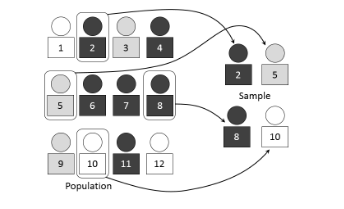
Sampling

Selecting a subset of individuals from a population to estimate characteristics of the whole.

Simple Random Sample (SRS)

Every subset of the population has an equal chance of being selected.

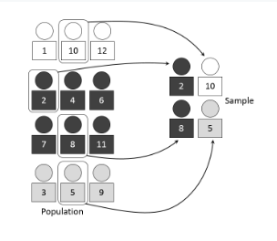
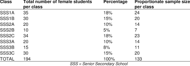
Stratified Sampling

Population divided into homogeneous strata (similar characteristics), and an is SRS taken within each stratum.

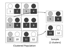
Cluster Sampling

Population split into clusters (naturally occurring groups); some clusters randomly chosen and all members studied.

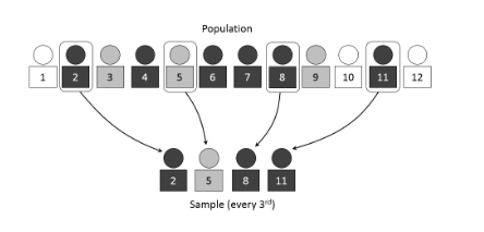
Systematic Sampling

Selecting every k-th element after a random start in an ordered list.

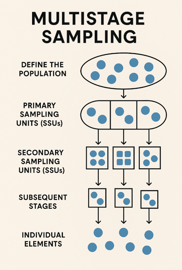
Multistage Sampling

Successive sampling of clusters within clusters until reaching the final sampling units.

Probability-Proportional-to-Size Sampling

Selection probability of each element is proportional to how big its subgroup is

Line-Intercept Sampling

Elements included if intersected by a pre-chosen line segment (transect). Used to measure any features that intersect a line, usually used in vegetation

Panel Sampling

Same sampled individuals are surveyed repeatedly over time.

Nonprobability Sampling

Sampling procedure where some population members have unknown or zero chance of selection.

Bias (Statistical)

Systematic tendency that skews results away from the true value.

Sampling Bias

Sample not representative because selection probabilities differ across population members.

Non-response Bias

When people respond to a poll or a survey differ meaningfully from non-respondents, distorting results. Also known as participation bias

Undercoverage Bias

Part of the population is systematically excluded from the sampling frame.

Self-selection Bias

Individuals decide themselves to participate, often those with strong opinions.

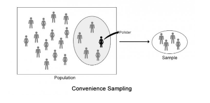
Convenience Sampling

Sample drawn from units that are easiest to access.

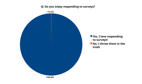
Voluntary Response Sampling

Participants volunteer to respond; prone to extreme opinions.

Quota Sampling

Like SRS but does NOT randomly select members to fill each quota. Instead, researchers fill quotas based on specific characteristics until they reach a predetermined number for each category, which can lead to bias.

Snowball Sampling

Existing participants recruit future participants, building a sample via referrals. This can cause bias through participants being more likely to refer people with similar opinions.

Experimental Factor

Variable that is deliberately manipulated by the researcher in an experiment.

Treatment

Specific combination of conditions applied to experimental units.

Block

A group of similar experimental units or observations that are grouped together to reduce variability in an experiment or analysis.

Experimental Unit

Smallest entity to which a treatment is independently applied. The thing being experimented on

Level (of a factor)

Specific setting, value, category, or just the name of an experimental factor (independent variable) that is being tested.

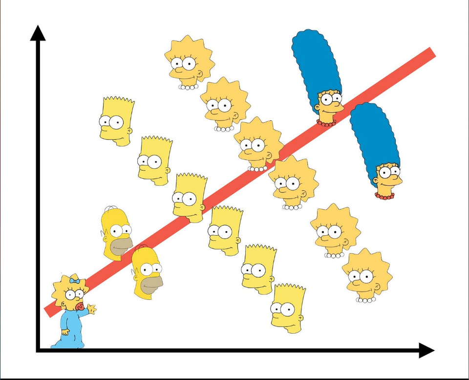
Simpson’s Paradox

Trend that appears in several groups that dissapears or reverses when groups are combined.

Gambler’s Fallacy

Belief that deviations from expected behavior must be corrected in the short run.

Hot-Hand Fallacy

Assuming a run of successes makes further success more likely. Also known as the Monte-Carlo fallacy.

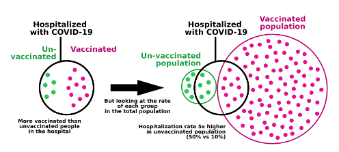
Base-Rate Fallacy

Ignoring relevant statistical information (base rates) when evaluating specific evidence.

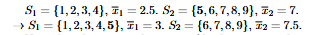
Will Rogers Phenomenon

Moving an observation from one group to another increases both groups’ averages. Also known as the Okie Paradox.

Berkson’s Paradox

A result that makes it seem that two unrelated variables appear to be correlated (usually negatively).

Nominal Data

Categorical data with no intrinsic ordering (e.g., eye color).

Ordinal Data

Categorical data with a meaningful order but unequal intervals (e.g., class rank).

Interval Data

Numeric data with equal intervals but no true zero (e.g., temperature °C).

Ratio Data

Numeric data with equal intervals and a true zero (e.g., weight).

Pie Chart

Circular chart where slice areas show category proportions.

Bar Chart

Rectangular bars represent categorical frequencies or values.

Mosaic Plot

Tile plot showing joint distribution of two (or more) categorical variables.

Scatter Plot

Graph of paired quantitative data; used to study relationships.

Histogram

Bar graph of binned numerical data frequencies.

Box Plot

Displays median, quartiles and potential outliers of numerical data.

Dot Plot

Dots along a number line show individual data points; good for small n.

Stem-and-Leaf Plot

Splits numbers into stems and leaves to display shape and raw data.

Line Graph

Connects data points with lines to show trends over time or sequence.

Normal Q–Q Plot

Plots data quantiles against theoretical normal quantiles to assess normality.

Residual Plot

Graph of residuals versus predicted values; checks model fit assumptions.

Ogive

Cumulative frequency curve of numerical data.

Least-Squares Regression Line (LSRL)

Line that minimizes the sum of squared vertical residuals.

Pearson Correlation Coefficient (r)

Measures strength and direction of linear relationship (−1 to +1).

Coefficient of Determination (r²)

Proportion of variance in y explained by x via the model.

Covariance

Average product of deviations of two variables; sign indicates relationship direction.

Residual (e)

Observed value minus predicted value (y – ŷ).

High Leverage Point

Observation with an extreme x-value relative to others.

Influential Point

Observation that markedly changes regression slope or intercept if removed.

Extrapolation

Predicting beyond the range of observed x; often unreliable.

Interpolation

Predicting within the range of observed x; usually reliable.

Homoscedasticity

Residual variance is constant across levels of the predictor.

Heteroscedasticity

Residual variance changes with the predictor; fan-shape pattern.

Sum of Squares Total (SST)

Total variability in y: Σ(yi – ȳ)².

Sum of Squares Regression (SSR)

Explained variability: Σ(ŷi – ȳ)².

Sum of Squares Error (SSE)

Unexplained variability: Σ(yi – ŷi)².

Probability Distribution

Function that assigns probabilities to all possible outcomes of a random variable.

Normal Distribution

Bell-shaped, symmetric continuous distribution described by μ and σ.

Empirical Rule (68-95-99.7)

For normal data, ~68 % within 1 σ, 95 % within 2 σ, 99.7 % within 3 σ.

z-Score

Standardized value: (x – μ)/σ; counts SDs from the mean.

Percentile

Value below which a specified percentage of observations fall.

Student’s t-Distribution

Symmetric distribution with heavier tails; used when σ unknown and n small (df = n–1).

t-Score

Standardized statistic using sample s and t-distribution.

Sampling Distribution

Probability distribution of a statistic over all possible samples of a fixed size.

Central Limit Theorem (CLT)

Sampling distribution of the mean approaches normal as n increases, regardless of population shape.

Law of Large Numbers

Sample mean converges to the population mean as sample size grows.

Uniform Distribution

All outcomes in an interval are equally likely.

Binomial Distribution

Counts number of successes in n independent Bernoulli trials with probability p.

Geometric Distribution

Counts trials needed to get the first success in repeated Bernoulli trials.

Chi-Square Distribution

Distribution of the sum of squared standard normals; parameter df (k).

Negative Binomial Distribution

Number of failures before r successes occur in Bernoulli trials.

Hypergeometric Distribution

Success count in draws without replacement from a finite population.

Poisson Distribution

Models number of events in a fixed interval given constant mean rate λ.

Confidence Interval

Interval estimate that likely contains the population parameter at a stated confidence level.

Confidence Level

Long-run proportion of CIs that capture the true parameter (e.g., 95 %).

Critical Value (z* or t*)

Cutoff on the reference distribution that matches the desired confidence level.

Margin of Error

Half-width of a confidence interval; (critical value) × (standard error).

Null Hypothesis (H₀)

Default claim that there is no effect or difference.

Alternative Hypothesis (Hₐ)

Claim of an effect or difference that we seek evidence for.

p-Value

Probability of observing a result at least as extreme as the sample, assuming H₀ is true.

Significance Level (α)

Threshold probability for rejecting H₀ (commonly 0.05).

Type I Error

Rejecting a true null hypothesis; false positive; probability = α.

Type II Error

Failing to reject a false null hypothesis; false negative.

Power (1 – β)

Probability of correctly rejecting a false null hypothesis.

Bayes’ Theorem

P(A | B) = P(B | A) · P(A) / P(B); updates probabilities with new evidence.