ML Interview -- Unsupervised Learning

What is maximum likelihood estimate?

Maximum Likelihood Estimation (MLE) is a statistical method used to estimate the parameters of a probability distribution or a statistical model. The core idea behind MLE is to find the parameter values that maximize the likelihood function, which measures how well the model explains the observed data.

In simpler terms:

Likelihood Function: It's a function that represents the probability of observing the given data under different parameter values.

Objective of MLE: To choose the parameters that make the observed data most probable.

Give an example of MLE?

Imagine we have a set of data points that we assume are normally distributed, but we don't know the mean and variance of this distribution. Using MLE, we can estimate these parameters by finding the values that maximize the likelihood of observing our data under the normal distribution.

Why is MLE important?

Consistency: As the sample size increases, MLE estimates converge to the true parameter values.

Efficiency: MLE makes the best possible use of the data, providing estimators with the lowest possible variance.

Asymptotic Normality: The distribution of MLE estimates approaches a normal distribution for large sample sizes, which simplifies hypothesis testing and confidence interval construction.

What is Gaussian Mixture of Models?

A Gaussian Mixture Model (GMM) is a probabilistic model used for clustering and density estimation. It assumes that the data is generated from a mixture of several Gaussian distributions, each characterized by its mean, variance (or covariance), and weight (mixing coefficient).

What are some key concepts in GMM?

Mixture of Gaussians: GMM combines multiple Gaussian distributions to model complex, multi-modal data.

Soft Clustering: Unlike hard clustering methods like k-means, GMM assigns probabilities (responsibilities) to each data point, indicating its likelihood of belonging to different clusters.

Parameters: Each Gaussian is defined by:

1. A mean (μ\muμ)—the center of the distribution.

2. A covariance matrix (Σ\SigmaΣ)—its spread and orientation. 3. A mixing coefficient (π\piπ)—the proportion of the data accounted for by that Gaussian.

Explain how GMM handles the clustering problem? What are some applications of GMM?

1. GMM introduces latent variables that represent the cluster membership of each data point. These are inferred probabilistically using the Expectation-Maximization (EM) algorithm.

2. GMM is widely used for tasks like soft clustering, density estimation, anomaly detection, and image segmentation. Its ability to model data with overlapping clusters makes it highly versatile.

Assumptions of GMM?

1. Data Is Generated from a Mixture of Gaussians:

GMM assumes that the data is generated by a mixture of several Gaussian (Normal) distributions, each with its own mean (μk\mu_kμk​) and covariance (Σk\Sigma_kΣk​).

This implies that the data forms clusters where each cluster follows a Gaussian distribution.

2. independent and identically distributed (i.i.d.) data points.

3.Number of Gaussian Components (KKK) Is Fixed.

MM requires the user to specify the number of Gaussian components (KKK) beforehand.

The model assumes that this KKK accurately reflects the true number of clusters or data sources.

4. Clusters follow Gaussian shapes.

5. Soft assignments are valid for cluster memberships.

6. The covariance structure is appropriately chosen.

7. There is sufficient data for parameter estimation.

8. The components are smooth and continuous.

Limitations of GMM?

1. Shape of Clusters:

GMM struggles when clusters are non-Gaussian, irregular, or non-elliptical.

Example: Data shaped like spirals or concentric circles.

2. Number of Components:

If K is not chosen correctly, GMM may underfit (too few components) or overfit (too many components).

3. Sensitive to Initialization:

Poor initialization of parameters (μk,Σk,πk\mu_k, \Sigma_k, \pi_kμk​,Σk​,πk​) can result in suboptimal solutions.

4. Outliers:

GMM can be sensitive to outliers, as they can disproportionately affect the means and covariances of the Gaussian components.

What is Expectation Minimization?

The EM algorithm is an iterative optimization technique used to estimate parameters in models where some data is hidden (latent) or missing.

It alternates between two steps:

1. Expectation (E-Step): Guess the hidden information (latent variables) based on the current parameters.

2. Maximization (M-Step): Update the model parameters to maximize the likelihood of the data, using the guessed hidden information.

Simple Analogy

Imagine trying to group people into teams (clusters) based on partial observations. In the E-Step, you estimate how likely each person belongs to each team. In the M-Step, you adjust the team characteristics (e.g., averages) based on these estimates. Repeat until the groups and assignments stabilize.

What is latent variables in GMM?

Latent variables in the context of Gaussian Mixture Models (GMMs) represent the responsibility that each Gaussian component (or cluster) takes for each data point. Here’s a detailed explanation to reinforce this idea

Latent variables in the context of Gaussian Mixture Models (GMMs) represent the responsibility that each Gaussian component (or cluster) takes for each data point. Here’s a detailed explanation to reinforce this idea:

What Do Latent Variables Represent?

Each data point xix_ixi​ is assumed to be generated by one of the K Gaussian distributions in the mixture.

The latent variable zi​ indicates which Gaussian (K) was responsible for generating xi. zi=K: Data point xi belongs to the k-th Gaussian.

What is Responsibility (soft membership) in the E step? And why is it important?

Since the exact Gaussian that generated xi is unknown, GMM assigns probabilities to reflect how likely each Gaussian is responsible for xi. These probabilities are called responsibilities and are denoted as rik:

rik​: The responsibility of the k-th Gaussian for the i-th data point.

This is computed in the E-Step of the EM algorithm.

Why are they important?

1. Soft Clustering:

Unlike k-means (hard clustering), GMM assigns soft probabilities instead of hard labels.

A data point can belong partially to multiple Gaussians based on its distance from their means and their spreads.

2. Parameter Updates:

In the M-Step, responsibilities are used to update:

A. Mixing coefficients (πk​): How much each Gaussian contributes overall.

B. Means (μk\mu_kμk​): Weighted by how much each data point belongs to the Gaussian.

C. Covariances (Σk​): Adjusted to reflect the spread of points belonging to the Gaussian.

How to choose the right k in GMM?

1. Start with BIC or AIC as they are the most appropriate for GMM due to the probabilistic framework.

Probabilistic models like GMMs allow for model selection criteria that penalize for increasing model complexity (KKK) to avoid overfitting. Two common criteria are:

2. Use Cross-Validation to validate the selected KKK.

3. If you're looking for an interpretable method, the Elbow Plot is a good starting point, but it can be subjective.

4. Use Silhouette Scores: (Measures the quality of clustering by comparing how similar a point is to its own cluster (cohesion) versus other clusters (separation).) or the Gap Statistic (Compares the within-cluster dispersion of the actual data to that of random uniform data.

A large "gap" suggests the clusters are well-separated.) for an additional perspective, especially if you're evaluating clustering quality.

What is k-means?

k-means is an unsupervised machine learning algorithm used for clustering, where the goal is to partition n data points into k clusters. Each cluster is represented by its centroid, and data points are assigned to the cluster with the nearest centroid.

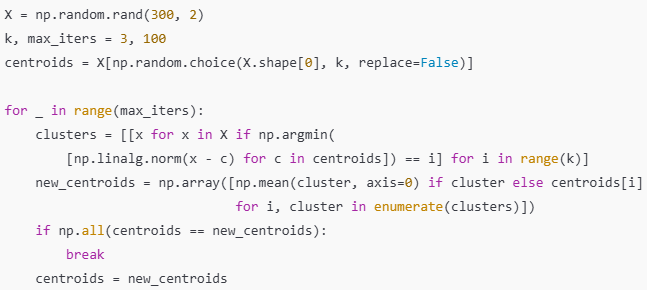
Key Steps of the Algorithm:

1. Initialization:

   • "Randomly select kkk points from the data as initial centroids."

2. Assignment Step:

   • "Assign each data point to the nearest centroid using a distance metric, typically Euclidean distance."

3. Update Step:

   • "Recalculate the centroids as the mean of all data points assigned to that cluster."

4. Repeat:

   • "Iteratively repeat the assignment and update steps until the centroids stabilize or the change in assignments is minimal."

What are key characteristics, advantages and limitations of k-means

Key Characteristics:

• "k-means assumes that clusters are spherical and of similar size."

• "It performs hard clustering, meaning each data point belongs to exactly one cluster."

• "The objective is to minimize the within-cluster sum of squared distances (WCSS), or the inertia."

Advantages:

• "It’s simple, fast, and easy to implement, making it suitable for large datasets."

• "Works well when clusters are well-separated and approximately spherical."

Limitations:

• "k-means requires the number of clusters (kkk) to be specified beforehand."

• "It’s sensitive to the initialization of centroids, which can lead to suboptimal solutions (mitigated by using techniques like k-means++)."

• "It struggles with non-spherical clusters and overlapping data."

How to implement k-means?

Difference between k-means, DBSCAN and GMMs

k-means, DBSCAN, and GMMs are all clustering algorithms but differ significantly in their approaches and use cases.

1. K-means is a distance-based algorithm that assumes clusters are spherical and requires kkk to be predefined. It's fast and works well for well-separated clusters but struggles with noise and non-spherical shapes.

2. DBSCAN is density-based, capable of identifying clusters of arbitrary shapes, and can handle noise, but it struggles with high-dimensional data and clusters of varying densities.

3. GMM is a probabilistic model that assumes data is generated from a mixture of Gaussians. It excels at overlapping or elliptical clusters and provides soft clustering, assigning probabilities to cluster memberships, but requires k to be predefined and is sensitive to initialization.

   The choice of algorithm depends on the data's structure and the specific requirements of the problem

How DBScan works?

DBSCAN is a density-based clustering algorithm that groups points into clusters based on the density of data points in their neighborhood. It identifies dense regions as clusters and treats points in low-density regions as noise or outliers.

Key Concepts

• Core Points:

  • "A core point has at least MinPts data points (including itself) within a radius ϵ\epsilonϵ."

• Border Points:

  • "A border point is within ϵ\epsilonϵ of a core point but doesn’t itself have enough neighbors to be a core point."

• Noise Points:

  • "Points that are neither core nor border points are labeled as noise."

What are the algorithms of DBSCAN?

Algorithm Steps:

1. Start with an Unvisited Point:

   • "Begin with a random point and check its neighborhood (points within ϵ\epsilonϵ)."

2. Cluster Formation:

   • "If the point is a core point, form a cluster by iteratively adding all density-reachable points."

3. Density Reachability:

   • "Points are density-reachable if they can be connected through a chain of core points within ϵ\epsilonϵ."

4. Handle Border and Noise Points:

   • "Border points are added to the nearest cluster, while noise points remain unclustered."

5. Repeat:

   • "Repeat the process for all unvisited points."

What are some strengths and limitations of DBScan?

Strengths:

• "DBSCAN can find clusters of arbitrary shapes, unlike k-means, which assumes spherical clusters."

• "It explicitly handles noise by labeling low-density points as outliers."

• "The number of clusters is determined automatically, so there’s no need to specify k."

Limitations:

• "DBSCAN struggles with clusters of varying densities because a single ϵ\epsilonϵ may not fit all clusters."

• "It can perform poorly in high-dimensional data because distance metrics like Euclidean distance lose meaning in high dimensions."

• "The results are sensitive to the choice of ϵ\epsilonϵ and MinPts."

What are the assumptions of DBSCAN, k-means and GMMs?

• DBSCAN assumes clusters are dense regions separated by low-density areas. It doesn’t assume specific shapes.

• k-means assumes clusters are spherical, equally sized, and separable by Euclidean distance.

• GMMs assume data is generated from a mixture of Gaussian distributions with varying shapes and overlaps.

How does each algorithm handle noise and outliers?

• DBSCAN explicitly labels points in low-density regions as noise.

• k-means assigns every point to a cluster, making it sensitive to outliers.

• GMMs include outliers probabilistically but don’t explicitly label them as noise.

What types of clusters are challenging for DBSCAN, k-means, and GMMs?

• DBSCAN struggles with varying densities and high-dimensional data.

• k-means struggles with non-spherical, overlapping clusters.

• GMMs may fail with non-Gaussian or highly irregular clusters.

Why does k-means struggle with non-spherical clusters, and how do GMMs address this limitation?

• k-means minimizes Euclidean distances, assuming spherical clusters.

• GMMs model clusters using Gaussian distributions with flexible covariance matrices, allowing elliptical shapes.

How do the distance metrics differ in k-means, DBSCAN, and GMMs?

• k-means: Euclidean distance for cluster assignment.

• DBSCAN: Density-based distance metrics, often Euclidean.

• GMMs: Mahalanobis distance via covariance matrices.

How do the computational complexities of DBSCAN, k-means, and GMMs compare?

• k-means: O(n×k×t), where t is iterations.

• DBSCAN: O(nlog⁡n) (with a spatial index) or O(n2)

• GMMs: Similar to k-means, O(n×k×t) but slower due to Gaussian calculations.

What happens if the hyperparameters (k, ϵ (epsilon), MinPts) are poorly chosen?

• k-means: Wrong kkk leads to underfitting or overfitting.

• DBSCAN: Small ϵ\epsilonϵ causes over-segmentation; large ϵ\epsilonϵ merges clusters or labels most points as noise.

• GMMs: Incorrect kkk leads to similar issues as k-means.

How does DBSCAN automatically determine the number of clusters?

It identifies clusters based on density. Core points in dense areas form clusters, and low-density points remain noise.

Explain the role of the covariance matrix in GMMs.

The covariance matrix defines the shape, orientation, and spread of each Gaussian component, enabling elliptical clusters.

Given a dataset with overlapping clusters, which algorithm would you choose and why?

GMMs: Soft clustering allows probabilistic assignment, making it ideal for overlapping clusters.

If you have a dataset with noise, would you choose DBSCAN over k-means or GMMs?

Yes, DBSCAN explicitly handles noise, while k-means and GMMs are sensitive to outliers.

How would you cluster a high-dimensional dataset?

Reduce dimensions (e.g., PCA) before applying GMM or k-means. DBSCAN struggles with high-dimensionality.

How would you handle varying densities in clusters?

DBSCAN struggles with varying densities. Use GMMs, which adapt to density via mixing coefficients.

Describe how you would decide between DBSCAN, k-means, and GMMs for a real-world application.

Choose DBSCAN for noisy, irregular shapes, k-means for simple, spherical clusters, and GMMs for overlapping, elliptical clusters.

How would k-means handle a dataset where all clusters have very different sizes?

Poorly. Larger clusters dominate, pulling centroids away from smaller clusters.

What would happen if DBSCAN's ϵ (epsilon) is too large or too small?

• Large ϵ\epsilonϵ: Merges clusters or labels most points as a single cluster.

• Small ϵ\epsilonϵ: Fragments clusters or labels most points as noise.

How can you adapt k-means to work better with non-spherical clusters?

Use kernel k-means, k-medoids, or switch to GMM.

In what scenarios could GMM overfit the data, and how can you prevent it?

Overfitting occurs with too many components. Prevent it using BIC/AIC or regularization.

How would you handle datasets where the true number of clusters is unknown?

Use BIC/AIC for GMMs, silhouette scores for k-means, or DBSCAN’s density-based approach.

f k-means fails to converge, what might be the problem, and how would you fix it?

• Causes: Poor initialization, bad scaling, or high-dimensionality.

• Fix: Use k-means++, normalize features, or reduce dimensions.

How would you evaluate the quality of clusters produced by these algorithms?

Use silhouette scores, Davies-Bouldin index, or log-likelihood (for GMMs).

ow would you modify DBSCAN to handle high-dimensional data?

Use a dimensionality reduction technique (e.g., PCA) before clustering.

What’s the impact of feature scaling on each algorithm?

Critical for k-means and DBSCAN (distance-based). Less critical for GMMs, but scaling helps.

How does GMM reduce to k-means under certain assumptions?

GMM reduces to k-means when covariances are spherical and equal across all clusters.

Can DBSCAN be adapted for probabilistic clustering like GMMs?

It’s difficult. Hybrid approaches like density-weighted GMMs can integrate density concepts.

How do k-means and GMM handle overlapping clusters differently?

k-means assigns points hard labels, ignoring overlap. GMMs assign probabilities, modeling overlap better.

What are the trade-offs between DBSCAN’s deterministic clustering and k-means’ stochastic nature?

DBSCAN is reproducible but depends on sensitive parameters (ϵ\epsilonϵ, MinPts). k-means is less reproducible but adaptive.

How would you optimize the hyperparameters for each algorithm?

• k-means: Use elbow plots or silhouette scores.

• DBSCAN: Grid search over ϵ\epsilonϵ and MinPts.

• GMMs: Use BIC/AIC or cross-validation.

What is Silhouette Scores?

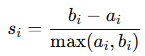
• The silhouette score measures how similar a data point is to its own cluster (cohesion) compared to other clusters (separation).

• For each data point iii, the silhouette score si​ is defined as (image). Where:

  • ai​: Mean intra-cluster distance (average distance to other points in the same cluster).

  • bi​: Mean nearest-cluster distance (average distance to points in the nearest cluster).

The overall silhouette score is the mean of si​ across all points.

Intuition

• si​ ranges from -1 to 1

  • si≈1: Point is well-clustered and far from other clusters.

  • si≈0: Point is on or near the decision boundary between clusters.

  • si<0: Point is poorly clustered; closer to a different cluster.

When to Use

• Works best for k-means and GMMs, where clusters are compact and well-separated.

• Less effective for DBSCAN or irregular cluster shapes.

Limitations:

• Computationally expensive for large datasets (O(n2)O(n^2)O(n2)) unless approximations are used.

• Assumes Euclidean distance, so results can be misleading for high-dimensional or non-Euclidean data.

How to use it?

• Use to assess cluster quality in k-means or GMMs.

• Plot silhouette scores across different KKK values to find the optimal KKK.

• A high silhouette score (e.g., > 0.7) suggests well-separated and cohesive clusters.

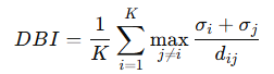
Davies-Bouldin Index (DBI)

• DBI measures the ratio of intra-cluster spread to inter-cluster separation. Lower values indicate better clustering.

• For KKK clusters, the DBI is computed as (image): Where:

  • σi​: Average distance between points in cluster i and the cluster centroid.

  • dij: Distance between centroids of clusters i and j.

Intuition

• Measures how tightly clusters are grouped (σi\sigma_iσi​) relative to how far apart they are (dijd_{ij}dij​).

• Smaller DBI values are better because they indicate compact clusters that are well-separated.

When to Use

• Suitable for k-means and GMMs, where centroids and compactness are meaningful.

• Works well for comparing results across different KKK values.

Strengths

• Automatically normalizes the spread and separation.

• Computationally efficient (O(K⋅n)) compared to silhouette scores.

Limitations

• Sensitive to noise and outliers.

• Assumes centroid-based cluster shapes, so less effective for irregular clusters (e.g., DBSCAN).

How to use it:

• Use for quick comparisons of KKK in k-means

or GMMs. Lower DBI values indicate better clustering.

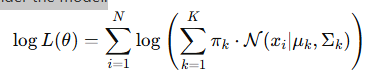
Log-Likelihood (for GMMs)

Log-likelihood measures how well the GMM fits the data. It is the logarithm of the likelihood of observing the data under the model (image) Where:

• πk: Mixing coefficient for cluster k.

• N(xi ∣ μk,Σk): Gaussian probability density for xi​ under cluster k.

Intuition:

• Higher log-likelihood values indicate that the GMM parameters (μk,Σk,πk​) explain the data well.

• If the log-likelihood keeps increasing significantly as KKK increases, it may indicate overfitting.

When to Use

• Exclusively for GMMs, as it leverages the probabilistic framework.

• Use in conjunction with BIC or AIC to balance fit and complexity:

  • BIC: Penalizes model complexity with log⁡(N) favoring simpler models.

  • AIC: Less strict penalty (+2p), allowing slightly more complex models.

Strengths

• Directly measures model fit.

• Useful for comparing GMMs with different numbers of components.

Limitations

• Cannot compare across different algorithms (specific to GMMs).

• Requires careful initialization to avoid local optima.

How to use:

• For GMMs, track the log-likelihood as KKK increases, but combine it with BIC or AIC to avoid overfitting.

• Plot log-likelihood alongside BIC/AIC to determine the optimal number of components.

• A steady increase in log-likelihood with small increments as k grows may indicate diminishing returns.

• The optimal k minimizes BIC/AIC while still providing a good log-likelihood.

What is AIC and BIC?

Akaike Information Criterion (AIC) and Bayesian Information Criterion (BIC) are statistical metrics used to evaluate and compare models, especially when fitting probabilistic models like Gaussian Mixture Models (GMMs). They help determine which model best explains the data while avoiding overfitting.

Why Do We Need Them?

When comparing models (e.g., GMMs with different numbers of components KKK), the likelihood (log⁡L\log LlogL) of the model increases as you add more parameters. This means larger models (more components) might fit the data better but risk overfitting.

• AIC and BIC penalize complexity, helping to balance:

  • Goodness of fit (likelihood) and

  • Model simplicity (fewer parameters).

Intuition for AIC

• AIC aims to find the model that minimizes information loss (how well the model captures the underlying data distribution).

  Formula: AIC=−2⋅log(L+2p)

  Where:

  • log⁡L: Log-likelihood of the model (fit to the data).

  • p: Number of parameters in the model.

• Key Idea:

  • Models with higher log-likelihoods (better fit) are rewarded.

  • Models with more parameters (more complexity) are penalized by 2p.

• When to Use AIC

  • Use AIC when your primary goal is prediction accuracy or when you suspect the true model is not in your set of candidate models.

  • AIC is less strict about penalizing complexity, so it may favor more complex models.

Intuition for BIC

BIC is derived from Bayesian probability principles and is more conservative than AIC. It seeks the model that is most likely to be the true model given the data.

Formula: BIC=−2⋅logL+p⋅logN

Where:

• log⁡L: Log-likelihood of the model.

• p: Number of parameters.

• N: Number of data points.

Key Idea:

• Similar to AIC, BIC rewards better fit (higher log⁡L) and penalizes complexity.

• However, the penalty for complexity (p⋅log⁡N) increases with the dataset size N, making BIC stricter than AIC.

When to Use BIC

• Use BIC when you suspect the true model is in your set of candidate models.

• BIC is stricter in penalizing complexity, so it often favors simpler models compared to AIC.

What is PCA?

"PCA, or Principal Component Analysis, is a dimensionality reduction technique used to find the most important directions (principal components) in high-dimensional data. These directions capture the maximum variance in the data while minimizing redundancy."

Why Use PCA?

• "PCA simplifies high-dimensional data into a smaller number of dimensions while retaining as much information (variance) as possible. It’s useful for visualization, noise reduction, and as a preprocessing step for machine learning models."

Key Concepts

• Principal Components:

  • "Principal components are new axes (directions) in the data, ranked by how much variance they explain. The first principal component captures the maximum variance, the second is orthogonal to the first and captures the next most variance, and so on."

• Dimensionality Reduction:

  • "Instead of using all original features, we project the data onto the top k principal components, reducing dimensionality while preserving most of the variance."

• Orthogonality:

  • "The principal components are uncorrelated (orthogonal) to each other, ensuring they capture unique patterns in the data."

How to calculate PCA?

• Standardize the Data:

  • "Ensure all features are on the same scale (mean = 0, variance = 1)."

• Compute Covariance Matrix:

  • "Find the covariance matrix to measure how features vary together."

• Find Eigenvectors and Eigenvalues:

  • "Eigenvectors give the directions of the principal components, and eigenvalues measure the variance along each direction."

• Sort and Select Components:

  • "Sort principal components by eigenvalues and select the top kcomponents that explain the most variance."

• Project Data:

  • "Transform the original data onto the new axes defined by the selected principal components."

Strengths and limitations of PCA?

• Strengths:

  • "Reduces dimensionality while preserving variance."

  • "Improves model efficiency by removing redundant features."

  • "Unsupervised, so it doesn’t require labels."

• Limitations:

  • "Linear method: PCA assumes the data lies in a linear subspace."

  • "Hard to interpret: Principal components are combinations of original features, losing interpretability."

  • "Variance doesn’t always equal importance for a task (e.g., labels in supervised learning)."

How would you decide how many principal components to keep?

• Use a scree plot (explained variance vs. components) and pick the elbow point.

• Retain components that explain a high percentage of the variance (e.g., 95%).

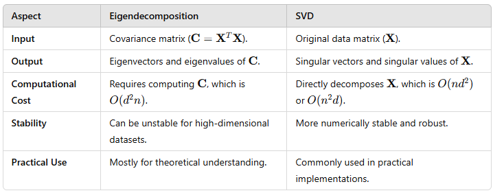
What’s the relationship between PCA and SVD (Singular Value Decomposition)?

PCA uses SVD to decompose the data matrix into principal components, eigenvalues, and eigenvectors.

How is PCA different from LDA (Linear Discriminant Analysis)?

PCA is unsupervised and maximizes variance. LDA is supervised and maximizes class separability.

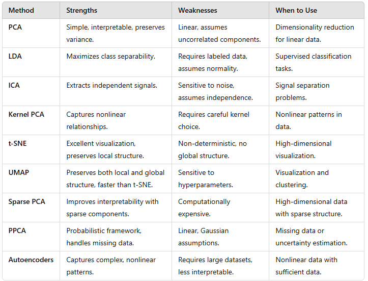
Alternatives to PCA

Linear Discriminant Analysis (LDA): A supervised dimensionality reduction technique that maximizes the separation between classes by finding linear combinations of features.

Independent Component Analysis (ICA): A method that separates data into statistically independent components, often used for signal processing (e.g., blind source separation).

t-Distributed Stochastic Neighbor Embedding (t-SNE): A technique for visualizing high-dimensional data by preserving local relationships in a low-dimensional space.

Uniform Manifold Approximation and Projection (UMAP):

A dimensionality reduction technique that focuses on preserving both local and global structure, often used as an alternative to t-SNE.