9. Linear Regression

Other Names for Response Variable 

Dependent Variable

Target Variable

Output Variable

Other Names for Explanatory Variable

Regressor

Independent Variable

Predictor Variable

Input Variable

Covariate

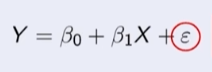
Simple Linear Regression Relationship

• \beta0 is the Y-intercept and \beta1 is the slope of the line.

• \varepsilon is the error, a random variable with constant variance. ( For population)

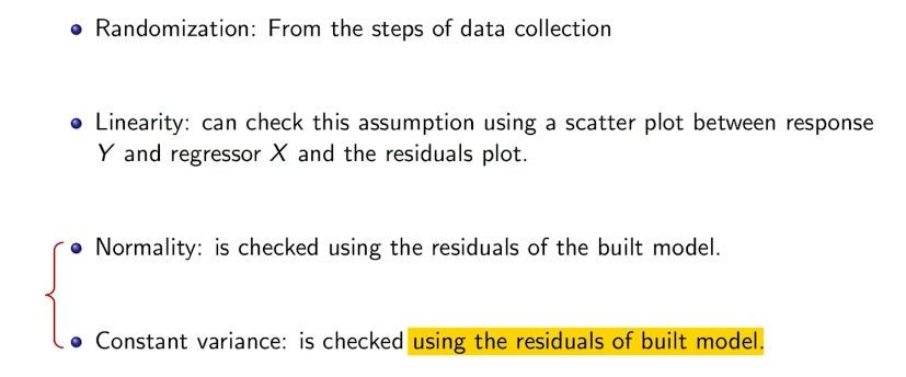
Assumptions for Linear Regression

• Data were obtained by randomization

• Relationship between X and Y is linear (Scatter Plot)

• \varepsilon must be normally distributed with mean of 0 and constant variance

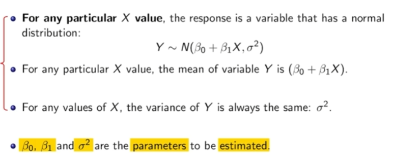
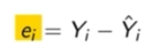
Error of the linear regression

stays constsant for any values of X

Ordinary Least Square Estimation

Square the difference between the actual and predicted response variable and compute the sum of them.

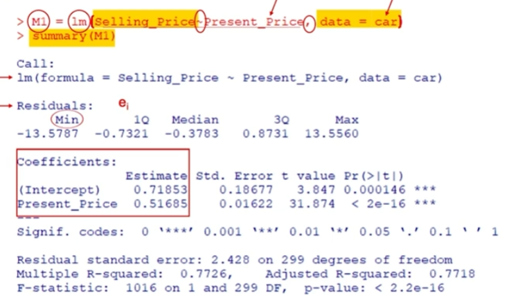
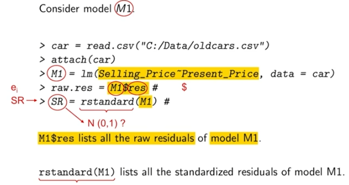
R Linear Model

lm = linear model

Response Variable: Selling_Price

Predictor Variable: Present_Price

\beta0 = 0.72, \beta1 = 0.52

y (hat) = 0.72 + 0.52x

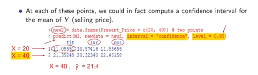
Point Estimation in R 

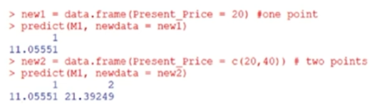
Interpolation

Estimating the mean response for an X value that had not been observed, but is within the ranged of observed values

Extrapolation

Estimating the mean response for an X value that is not within the range of observed values

We do not know the form of the relationship outside of our sample, so we shuold avoid

Point Estimate of Varariance

Interval Estimates

Point estimate +- margin of error (Quantile * SE of point estimate)

Quantile = t distribution, df = n-2

Interval Estimates in R for Coefficient

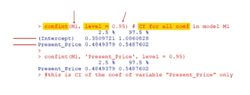
interval Estimates in R

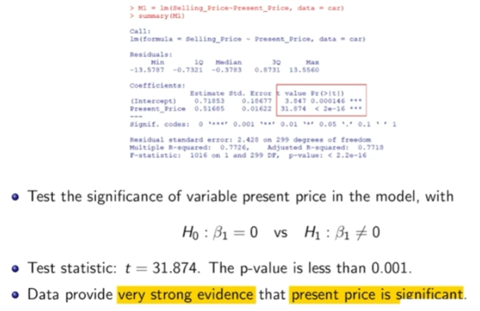
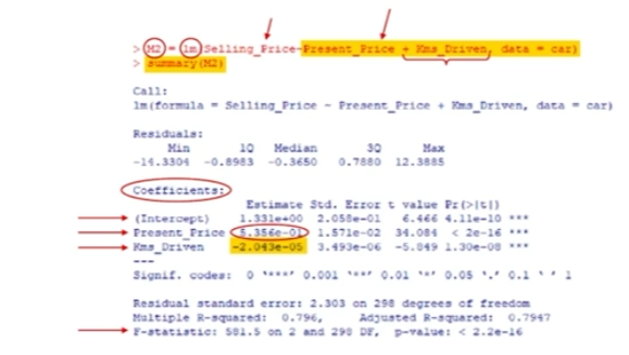
T Test

Test significance of one regressor (coefficient) can also be the independent test for one regressor and the response variable

R Output T-Test

For a simple linear regression model, the T test is equivalent to F test 

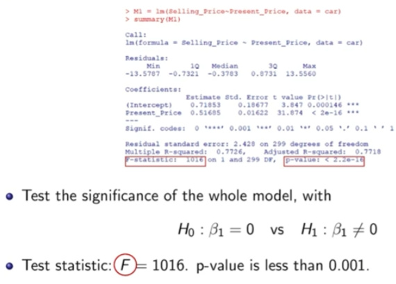
F Test

Test significance of the whole model

F Test Hypothesis

Null Hyphothesis: Model is not significant
Alternative Hypothesis: Model is significant

R Output F-Test

R formula for P distribution: pf(1016,1,299,lower.tail = F)

Df1 = No of Coefficents = 1

Df2 = n - No of Coefficent - 1

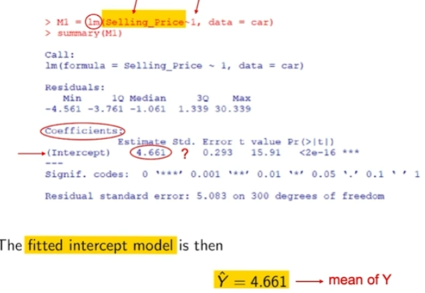
When F-Test is not significant

All regressors are not significant and we should use a intercept model

R code for intercept model

Regression Diagnostics

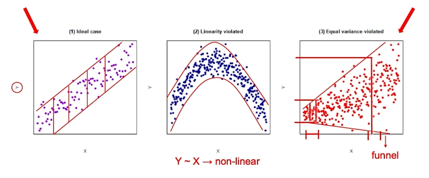
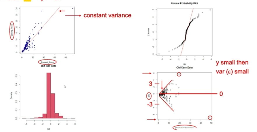
Checking Linearity and Variance

Use Scatter plot and draw top and bottom lines

2. Fix X via adding higher order element

3. Transform y by doing log(y) or 1/y

Residual Plots

• Check the normality of the assumption

• Check for non-constant variance and the need to transform Y

• Check for the need to add higer order terms in X

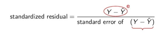
Standardised Residuals

The distribution should follow a standard distribution since the residuals follows a normal distribution.

R output Residuals

Checking Normality of Residuals

Creating a histogram plot or QQ-Plot of the Standardised Residuals and checking if they are in a standard distribution

Analysing Residual Plots

• Plot SR against Y and X: Scattered around 0 within (3,-3)

• Histogram and QQ plot of SR Normally Distirbuted

• SR from fitted model are not independent but when sample size is large enough randomness should be seen

Common Issues in Residual Plots

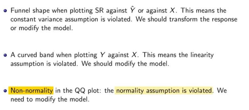
Funnel in scatter plots

Curved band in X against Y

Non-normality in the QQ plot

R Output

Model does not satisfy the constant assumption and the normality assumption

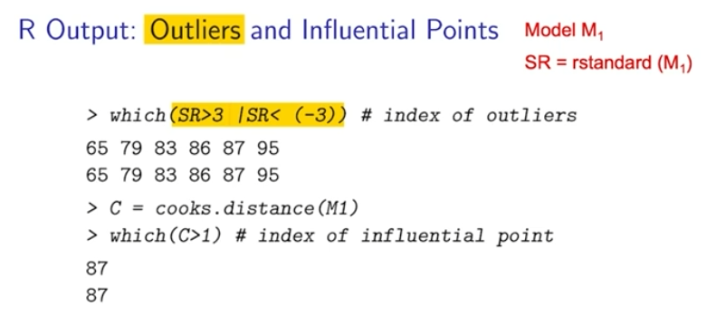
Outliers 

• Identified by the residuals

• The standardised residuals greater than 3 or lesser than -3

• Investigate outliers

Influential Point

A point that greatly affects the parameter’s estimate

Points with cooks distance > 1 is influential

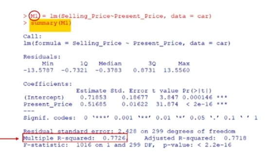
Coefficient of Determination R²

Check the goodness of fit of the model, between 0 and 1

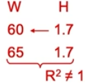
Simple Model Correlation

Equivalent to the square root of the coefficient of determination.

When correlation is negative, the equivalent relation is also negative.

R² weakness

The complexity of the model is not taken into consideration when explaining the goodness of fit of the model.

MLR vs SLR

1. Method of significant tests for categorical variable with more than 2 categories

2. Use adjusted R² to compare models

R Code for MLR

+ <Variable>

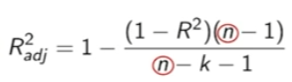
Adjusted R²

Takes into account the number of regressors included

K: number of regressors

n: number of samples

This enables us to compare the fit of 2 models with different number of variables

Indicator Variable

Changing categorical variables to integers

Variable vs Regressor

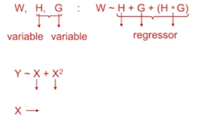
R output for Indicator Variables

X2 cant be removed as the interaction term of X1 and X2 is highly significant. To keep the interaction term, the main terms must be kept.

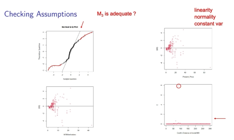
Checking Assumptions

Fitted model does not meet the assumptions

we can try to transform the variables or refit the model without the influential point

Need to Know

• Test for significance of regressor

• Fit a model in R and to write down a fitted regression

• Check assumptions of a regression analysis unsing residual plots

• Identity outliers and influential points

• Interpret coefficients and R²

• Compare the fit of models for the same reponse using R²