Statistics 2 Lecture 2

Process of hypothesis testing

• Formulate an hypothesis: What do you expect?

• Check study characteristics and variables: Sampling procedure, (experimental) design, measurement levels

• Descriptive analyses: What are the sample characteristics, how are the relevant variables distributed (inc. M and SDs)?

• Inferential analyses: Test a relation or differences, including a check of the model diagnostics.

• Interpret and report results: Report your findings in APA style.

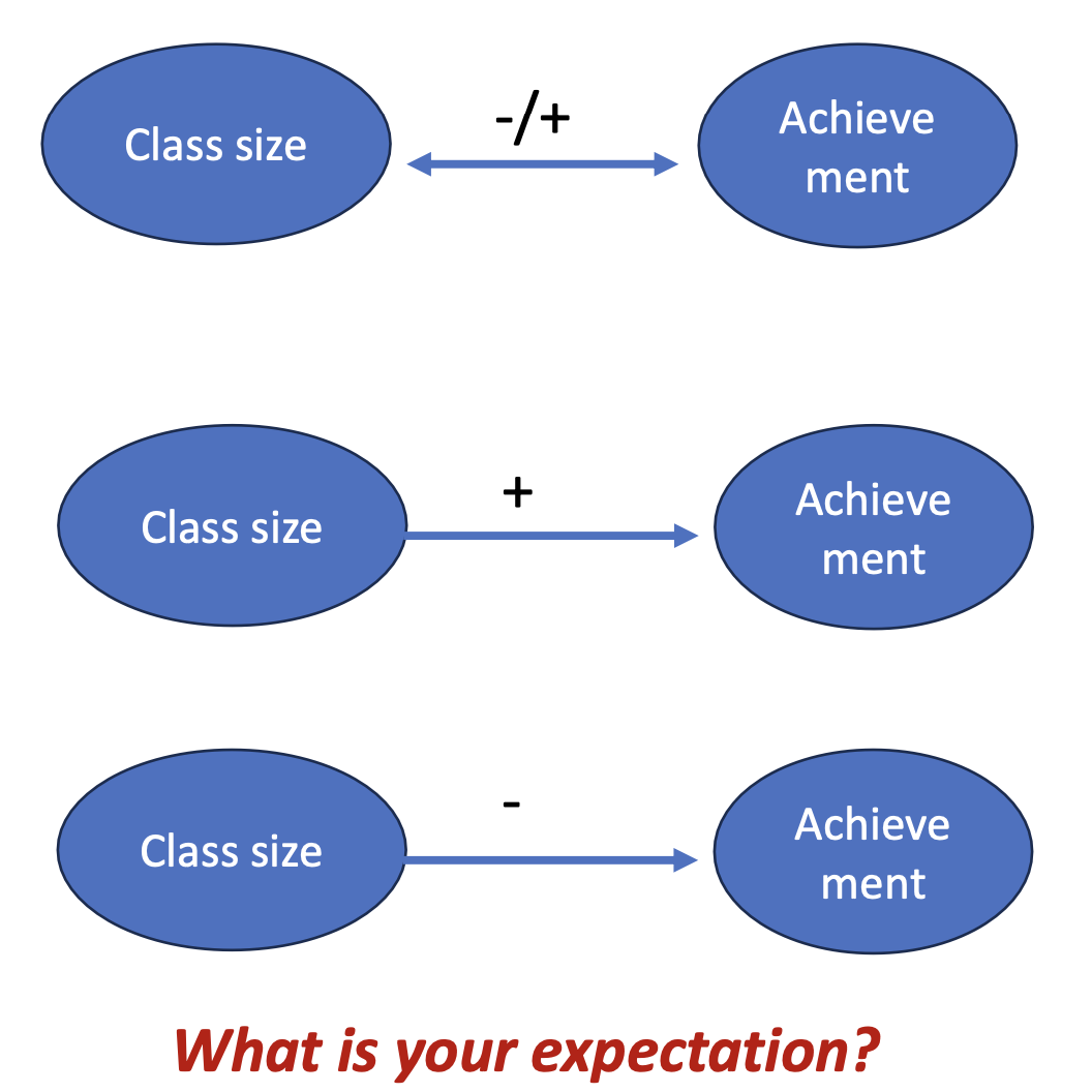
Formulate an hypothesis

• RQ: Is class size associated to academic performance?

• Non-directional:

  • x predicts y →Class size is associated with study performance

• Directional:

  • Positive association: Higher x predicts higher y (and vice versa)

  • → Average performance increases when class size increases

  • → Average performance decreases when class size decreases

• Negative association: Higher x predicts lower y (and vice versa)

• → Performance is typically better in smaller classes

• → Performance is typically worse in larger classes

Check study characteristics and variables

• RQ: Is class size associated to academic performance?

• Cross-sectional study → across randomly selected schools in the Netherlands

• Class size: Measured as the average class size in a school

  • → Predictor

  • → Quantitative

• Academic performance: School’s average grade on a standardized test

  • → Criterion (outcome)

  • → Quantitative

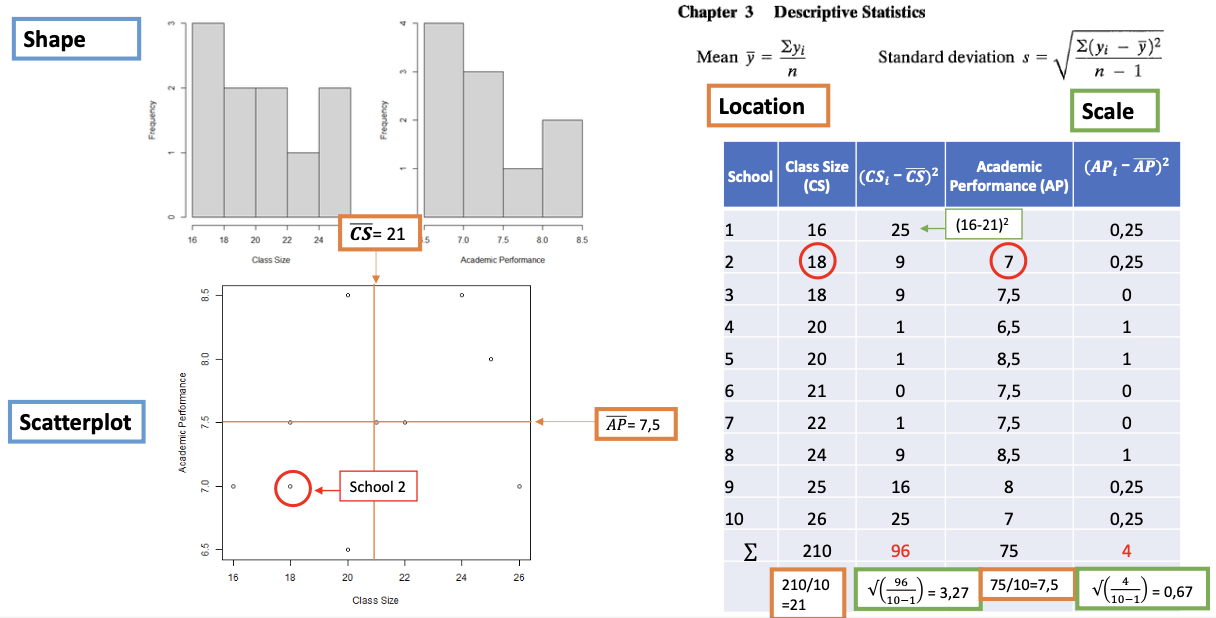
Descriptive statistics

• Univeriate descriptives describe single variables

  • Shape: bell-shaped (skewed/uniform/bimodal)

  • Location: Mean (Median/Mode)

  • Scale: Standard deviation (SD) or Variance (min/max)

• Scatterplots visualize the association between response (y) and explanatory (x) variables:

  • Every dot is an observation

  • Inspect: Is a linear model (𝑦ො = 𝑎 + 𝑏𝑥) appropriate to describe the association?

    • I.e.,does fitting a straight-line make sense?

• Yes? We can use Least square estimation to estimate the linear prediction equation.

• →This is the best straight line, falling closest to all data points in the scatterplot.

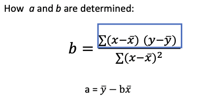
The linear prediction equation

• y = a + bx

• y = predicted criterion value

• 𝑎 = y-intercept → Expected Y value when x = 0

• 𝑏 = slope →Average change in y for a one-unit increase in x

• Association between response (y) and explanatory (x) variable can be

• Positive (𝑏 > 0): → Higher values of x tend to coincide with higher values of y

• Negative (𝑏 < 0) → Higher values of x tend to coincide with lower values of y

• Non-existing (𝑏 = 0) →no association between x and y

Least square estimation of linear model

• This is the best straight line, falling closest to all data points in the scatterplot

• b is positive when low x values often coincide with low y-values, and high x-values coincide with high y-values

• b is negative when low x-values coincide with high y-values, and high x-values coincide with low y-values

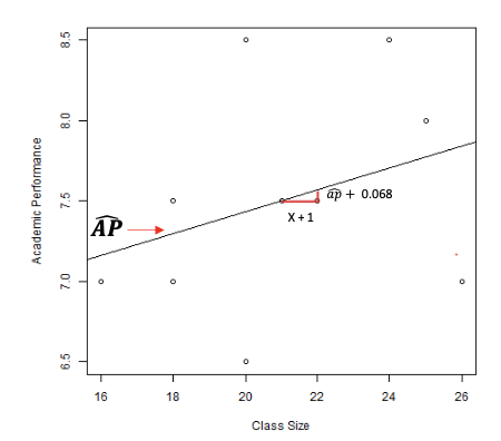
Interpreting the regression parameters

• RQ: Is class size associated to academic performance?

• Variables

  • x = Class size

  • y = Academic Performance

• AP = 6.072 + 0.068*CS

• Parameters:

  • 𝑎 = 6.072

  • → Expected academic performance when for schools with an average class size of 0 is 6.072

  • → Extrapolation beyond the data: NOT meaningful!

  • 𝑏 = 0.068

  • → Schools with larger classes on average perform better!

  • → For each 1-student increase in average class size, academic performance is on average 0.068 higher.

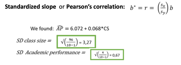
Interpreting the magnitude of regression coefficient b

• Caution: We typically cannot use b to interpret the strength of the association between x and y!

• → b depends on the scale at which x and y are measured e.g., a unit increase in seconds is much less than a one-unit increase in hours

• Solution: Inspect the effect size (a scale-free measure of association)

• Rules of thumb for interpretation: 0 < negligible < .10 ≤ small < .30 ≤ moderate < .50 ≤ large

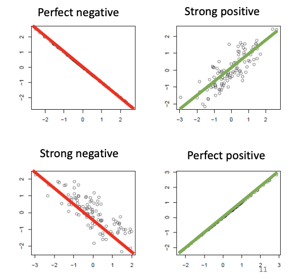
• Some facts about 𝑟:

  • r is always between -1 and 1

  • r has the same sign as b:

    • r < 0 when b < 0; 𝑟 = 0 when b = 0; r > 0 when b > 0

  • 𝑟 = -1 or 1 when x predicts y perfectly: There are no residuals

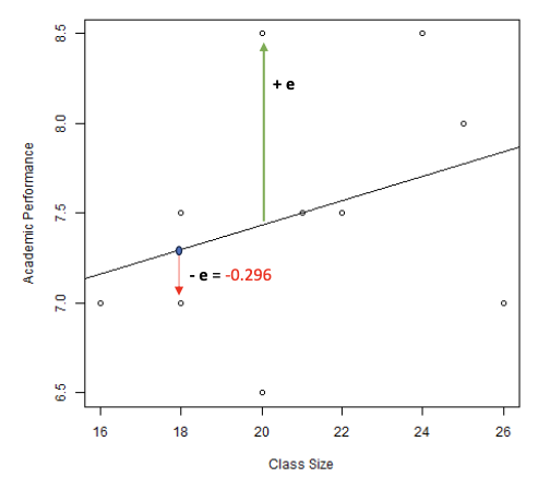
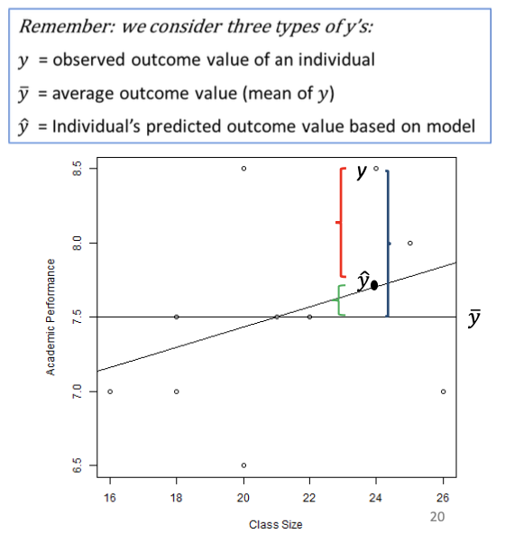
Predictions are not perfect: Predicted scores and residuals

• Variations exists around predicted scores y

• y = a + bx → y = a + bx + e

• Predicted scores differ from observed scores by e (residual)

• → Vertical distance between observed y and predicted y

• Some positive, some negative but on average 0

• We can use these residuals to determine how well the model performs in predicting y

Variation on the regression model

• For any model we discuss in this course, we can distinguish three types of variation:

• Total variation in Y: Total Sum of Squares: TSS = ∑ (𝑦 − 𝑦ത)2 (observed - mean)

  • Also named ‘marginal variation’

• Variation in Y that is not explained by the model Sum of Squared Errors: SSE = ∑ (𝑦 − 𝑦ො)2 (observed - predicted)

  • Also named ‘conditional variation’

• Variation in Y that is explained by the model: Regression Sum of Squares: RSS = ∑ (𝑦ො − 𝑦ത)2 (predicted - mean)

• Note: SSE + RSS = TSS!

• We can use these different ‘sums of squares’ to inspect how well our prediction model performs.

(Explained) Variation in the regression model

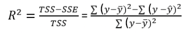
• Another measure of effect size is R2

• For simple regression, R2 is the square of Pearson’s correlation coefficient (r)

• R2 expresses the proportional reduction in error from using the prediction equation instead of the sample mean y to predict y

• Better understood as the ‘proportion of variation in y that is explained by the model’.

• Rules of thumb for interpretation: 0 < negligible < .02 ≤ small < .13 ≤ moderate < .26 ≤ large

• R2 falls between 0 and 1

  • R2 = when b is 0: The predictor variable has no explanatory power

  • R2 = 1 when the model predicts y perfectly

• The larger R2, the better the model predicts y

Inferential statistics

• Using sample data to make inferences about population parameters

• We cannot confirm any hypotheses, but we can falsify → By inspecting the probability of finding b (or r) when the null hypothesis (H0) were true

• HA: β ≠ 0 (if directional: β > 0 or β < 0)

• →There is an association between class size and performance

• → Same as saying population r ≠ 0 or r2 = 0

• H0: β = 0

• → There is no association between class size and

  performance

• → Same as saying population r = 0 or r2 = 0

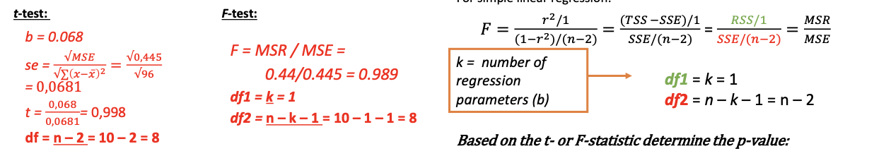
Inferential statistics: Two options to test hypothesis

• Check the significance of b using the t-statistics

• Check the significance of r2 using the F-statistic

  • Based on the t- of F-statistic determine the p-value → What is the probability of finding a result this extreme, when the H0 were true

• F = t2: Both options yield the same conclusion

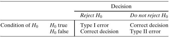
Inferential statistics: Decision making

• Four scenarios are possible, depending on our decision and the condition of the H0.

  • 2x erroneous decision (which we want to avoid)

  • 2x correct decision

• Type 1 error rate: Probability of rejecting the H0 when the H0 is true

• Determined by the selected 𝛼-level. → In our research area (and this course) we typically use 𝛼 = .05 (5%)

• If observed p-value < 𝛼 : Reject H0

• Type 2 error (𝛽): Probability of not rejecting the H0 when the H0 is false

• Determined by:

  • The strength of the association (or difference) in the population

  • The sample size of the study

  • The selected 𝛼-level

• → There is a trade-off: The smaller the selected Type 1 error rate, the larger the obtained Type 2 error rate!

Assumptions of the linear regression model

• For valid conclusions, the following assumptions should hold

  • Analyses are based on random sample → representativeness (crucial)

  • The relations between y and x is linear → functional form (crucial)

  • The conditional variance around b is equal for all x → homoscedasiticity of residuals (other estimators available)

  • The conditional variance of y for all x is normal → normal distributed residuals (large sample size important: central limit theory)

Results of the Linear Regression Model

• A Model Summary table: Provides information about the proportion of variation in y that is explained by the model

• An ANOVA table: Provides information about the decomposition of the variation in Y and the significance of the model.

• A Coefficients table: Provides information about the regression parameters (a and b)

• Some tables (here the model summary and coefficients table) include information about two models:

  • H0: The null hypothesis model (here, not including Class Size as predictor)

  • H1: The alternative hypothesis model (here, including class size as a predictor) → Our focus!

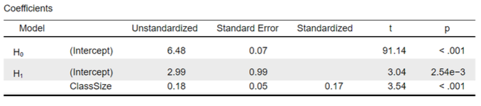
Coefficient table shows:

• The constant (intercept, a) is 2.99

  • This is the predicted academic performance (𝑦ො) in schools with a class size (x) of 0.

  • Note. for the H0 model, the intercept is 6.48. Which is the average academic performance in the sample (𝑦ത).

• The coefficient for ClassSize (b) is 0.18

  • The coefficient is positive. When class size increases by 1 student, we expect academic performance to be 0.18 higher.

• The t-statistic for ClassSize is 3.54

  • Calculated as b/se = 0.18/0.05

  • With df = n – 2 = 400 – 2 = 398, this yields p < .001.

    • →statistically significant (when using 𝛼 = .05).

  • The coefficient for ClassSize thus differs significantly from zero

  • We can reject the H0 that class size and academic performance are not related (H0: 𝛽 = 0).

• The standardized coefficient (𝑟 or 𝑏∗) is

  • For a 1 SDs increase in class size, we expect school’s academic performance to increase by 0.17 SDs.

  • This is considered a small effect size.

The ANOVA table shows:

• RSS (Regression sums of squares) = 24.60

  • Variation in y that is explained by the model.

  • df1 = p = 1

  • Thus: MSR = 24.60 / 1 = 24.60

• SSE (Sums of squared errors [residuals]) = 781.24

  • Variation in y that is not explained by the model.

  • df2 = N – 2 = 400 – 2 = 398
    Thus: MSE = 781.24 / 398 = 1.96

• TSS (Total sum of squares) = 805.84

• Note that: TSS/(N-1) = 805/399 = Total mean square = 𝑠2 = 2.02 = 1.422 = variance in 𝑦 𝑦

• The F-test for ClassSize is 12.53

  • Calculated as MSR/MSE = 24.60/1.96

  • With df1 = 1 and df2 = 398, this yields p < .001

  • →statistically significant (when using 𝛼 = .05)

  • The model thus explains a significant portion of variation in academic performance.

  • Note. For simple regression, 𝐹 = 𝑡2: 12.53 = 3.542

• MSR: How much variation is explained per (additional) predictpr in the model?

• MSE: How much variation can on average be explained by each additional predictor that we, given the sample size, could potentially add to the model

• F = ratio of the two. When F > 1: the additional predictor(s) explain more variation in y than is expected from any randomly selected predictor(s)

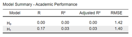
The model summary shows:

• 𝑅2 is .03

• Calculated as SSR/TSS = 24.60 / 805.84
  Thus: About 3% (a small portion) of the variation in academic performance across schools is explained by class size.

• Note. R (the square root of 𝑅2) is 0.17, which is the same as the standardized coefficient: The correlation coefficient.

• This only holds for simple regression!