Chapter 13 - Exponential Functions and Logarithms

Logarithm master in a nutshell!

What is a power, base, and exponent?
List the index laws and key rules for powers.

• A power is written as aⁿ, where:

  • a is the base (non-zero)

  • n is the exponent or index

Index Laws (for a, b ≠ 0 and integers m, n):

1. aᵐ × aⁿ = aᵐ⁺ⁿ

2. aᵐ ÷ aⁿ = aᵐ⁻ⁿ

3. (aᵐ)ⁿ = aᵐⁿ

4. (ab)ⁿ = aⁿ × bⁿ

5. (a/b)ⁿ = aⁿ ÷ bⁿ

Special rules:

• a⁰ = 1 (for a ≠ 0)

• a⁻ⁿ = 1/aⁿ, and 1/a⁻ⁿ = aⁿ

• 0ⁿ = 0 for n > 0, but 0⁰ is undefined

What does a^(1/n) mean?
How do index laws extend to rational indices?

• For a > 0 and n ∈ ℕ:
  a^(1/n) = the n-th root of a → a^(1/n) = ⁿ√a
  So: (a^(1/n))ⁿ = a

• Special cases:

  • 0^(1/n) = 0

  • If n is odd and a < 0, a^(1/n) is defined (result is negative)

Extended Index Laws:

1. a^(m/q) × a^(n/p) = a^(m/q + n/p)

2. a^(m/q) ÷ a^(n/p) = a^(m/q − n/p)

3. (a^(m/q))^(n/p) = a^[(m/q) × (n/p)]

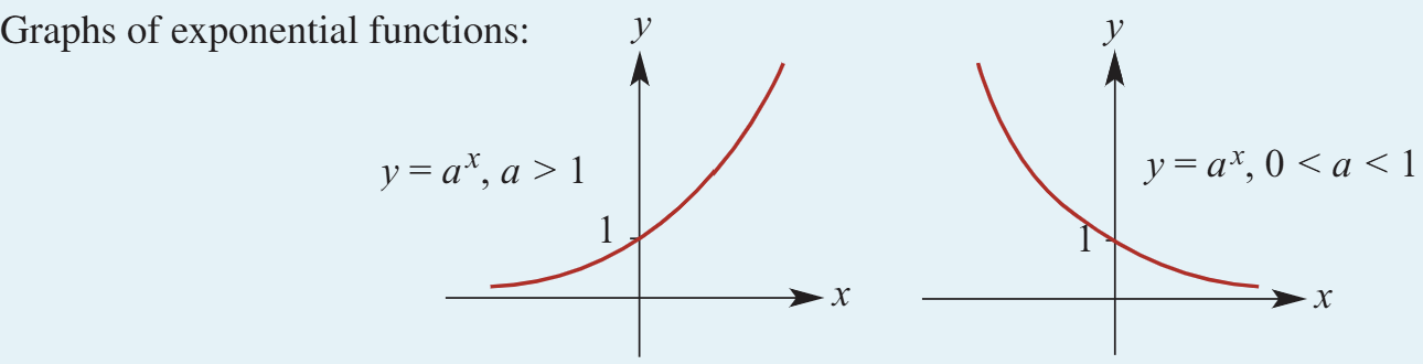
Exponential Functions & Transformations

• For y = aˣ where a > 1, the graph has:

  • The x-axis as an asymptote.

  • A y-intercept at (0, 1).

  • Positive y-values with no x-axis intercept.

  • All graphs of this form are dilations of each other from the y-axis.

• For y = aˣ where 0 < a < 1, the graph decays similarly but reflects the opposite behavior.

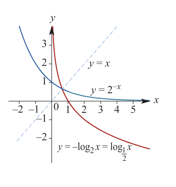
• If f(x) = aˣ and g(x) = a⁻ˣ, then g(x) is the reflection of f(x) in the y-axis.

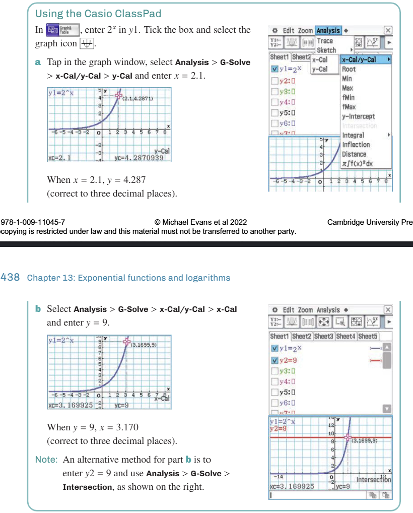
CAS: Sketching Logarithm Graphs

Solving Exponential Inequalities

To solve an exponential equation without a calculator, express both sides with the same base and equate the exponents (since aˣ = aʸ implies x = y for any base a > 0, a ≠ 1).

Example: 2ˣ+1 = 8 → 2ˣ+1 = 2³ → x + 1 = 3 → x = 2.

To solve an exponential inequality, follow the same method as an equation and apply the appropriate property:

If aˣ > aʸ, then:

• x > y when a > 1

• x < y when 0 < a < 1.

Example: 2ˣ+1 > 8 → 2ˣ+1 > 2³ → x + 1 > 3 → x > 2.

Laws of Logarithms

• For a ∈ R⁺ \ {1}, the logarithm function base a is defined as follows:
  aˣ = y is equivalent to log_ay = x.

• The expression log_ay is defined for all positive real numbers y.

• To evaluate log_ay, ask the question: "What power of a gives y?"

Laws of Logarithms:

1. log_a(mn) = log_am + log_an

2. log_a(m/n) = log_am - log_an

3. log_a(mᵖ) = p log_am

4. log_a(m⁻¹) = − log_am

5. log₁/ₐ(x) = −logₐ(x)

Examples:

• log₅ 1 = 0 and log_aa = 1

Using logarithms to solve exponential equations and inequalities

Key Concepts:

• Logarithmic Relationship:
  For a, b, c > 0, where a ≠ 1 and b ≠ 1, we have:
  loga c = (log_bc) / (log_ba).

• Logarithms and Exponentials:
  If a ∈ R⁺ \ {1} and x ∈ R, then:

  • a^x = b ⇔ log_ab = x.

  This property is useful for solving exponential equations and inequalities.

• Examples:

  • 2ˣ = 5 ⇔ x = log₂ 5.

  • 2ˣ ≥ 5 ⇔ x ≥ log₂ 5.

  • (0.3)ˣ = 5 ⇔ x = log₀.₃ 5.

  • (0.3)ˣ ≥ 5 ⇔ x ≤ log₀.₃ 5.

---

Examples of Solving Exponential Equations:

• Solve 2ˣ = 11:
  x = log₂ 11 ≈ 3.45943.

• Alternative Method:
  Taking log₁₀ of both sides:

  • log₁₀(2ˣ) = log₁₀ 11

  • x log₁₀ 2 = log₁₀ 11

  • x = log₁₀ 11 / log₁₀ 2
    Thus, log₂ 11 = log₁₀ 11 / log₁₀ 2.

• Solve 3²ˣ⁻¹ = 28:

  • 2ˣ - 1 = log₃ 28

  • 2ˣ = 1 + log₃ 28

  • x ≈ 2.017.

• Solve the inequality 0.7ˣ ≥ 0.3:
  Taking log₁₀ of both sides:

  • x log₁₀ 0.7 ≥ log₁₀ 0.3

  • x ≤ log₁₀ 0.3 / log₁₀ 0.7

  • x ≈ 3.376 (direction of inequality reversed since log₁₀ 0.7 < 0).

  Alternatively, solve as:
  x ≤ log₀.₇ 0.3.

---

Exponential Graphs and Logarithms:

• Graph of f(x) = 2 × 10ˣ − 4:

  • Horizontal asymptote at y = −4 as x → −∞.

  • The y-axis intercept is f(0) = −2.

  • The x-axis intercept occurs when f(x) = 0:

    • 2 × 10ˣ − 4 = 0 → x = log₁₀ 2 ≈ 0.3010.

📊 Properties of Exponential vs Logarithmic Functions

Property	y = aˣ (Exponential)	y = logₐx (Logarithmic)
Domain	ℝ	ℝ⁺ (x > 0)
Range	ℝ⁺ (y > 0)	ℝ
Key Point	a⁰ = 1	logₐ1 = 0
End Behavior	x → −∞, y → 0⁺	x → 0⁺, y → −∞
Asymptote	y = 0	x = 0

🔄 Transformations Summary (General Form)

Type	Example	Effect
Shift Right	y = logₐ(x − h)	→ right h units
Shift Left	y = logₐ(x + h)	→ left h units
Shift Up	y = logₐ(x) + k	↑ up k units
Shift Down	y = logₐ(x) − k	↓ down k units
Stretch (vertical)	y = a·logₐ(x), a > 1	↑ vertical stretch by factor a
Compress (vertical)	y = a·logₐ(x), 0 < a < 1	↓ vertical compression by factor a
Horizontal Compress	y = logₐ(bx), b > 1	→ compress across y-axis (divide x by b)
Horizontal Stretch	y = logₐ(bx), 0 < b < 1	→ stretch across y-axis (multiply x by 1/b)
Reflect in x-axis	y = −logₐ(x)	↩ reflect in x-axis
Reflect in y-axis	y = logₐ(−x)	↪ reflect in y-axis

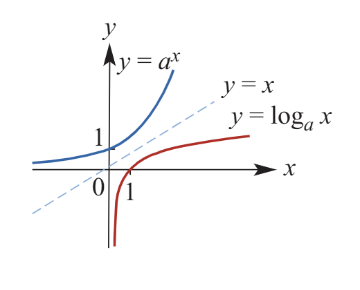
🔁 Inverse Functions:

y = a^x ↔ y = logₐx
↔ Reflect across the line y = x

If a > 0 and a ≠ 1, then:

• logₐ(aˣ) = x for all real x

• a^(logₐx) = x for all positive x

Exponential Modelling (General)

In exponential change, let A be the quantity at time t. The general formula is:

• A = A₀ bᵗ,

  where A₀ is the initial quantity and b is a positive constant.

  • If b > 1, the model represents growth, such as:

    • Growth of cells

    • Population growth

    • Continuously compounded interest

  • If b < 1, the model represents decay, such as:

    • Radioactive decay

    • Cooling of materials

Application and Variants of the Model

• Cell Growth Formula:
  For bacterial growth, the formula N = N₀2^(t/T_D) is used, where Tᴰ is the generation time.

• Radioactive Decay Formula:
  The formula A = A₀ 2⁻ᵏᵗ describes radioactive decay, where k is the decay constant. Half - life may be used to model this (A = A₀(1/2)ⁿ)

• Population Growth:

• It is sometimes possible to model population growth through exponential models, depending on the case.

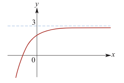
Limiting Values

In some exponential functions, a limiting value L is approached but never reached. Using the concept of limit, the formula for this behavior can be written as:
lim (x → ∞) f(x) = L,
where f(x) approaches L as x increases but never actually reaches it.

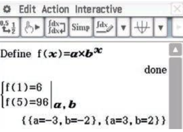
CAS: Determining Rules

1. Define f(x) = a × bx.

2. Solve the simultaneous equations (in example).

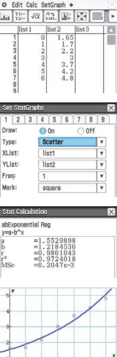
CAS: Fitting Data (Example)

• Enter the data into List1 and List2.

• Set the graph type to Scatter and assign List1 and List2 to the graph.

• Tap Set to display the scatter plot.

• Select Calc > Regression > abExponential Reg and tap OK to confirm.

• The exponential function w = 1.55(1.22)ᵐ models Somu’s weight.

• Tap OK to view the graph of the regression curve.