Applied econometrics lectures 9-10 - Limited dependent variables

LDV defenition

A dependent variable is limited if the values it can take are restricted

LDV in practice

Most economic variables are limited, but they do not all need special treatment – we may treat them simply as continuous.

• e.g. many cannot be negative (GDP)

It is only when the restriction is substantial that applying OLS (or other linear estimation) leads to problems

Why LDVs cause problems

We use dummy variables as the dependent variable

How to correct LDV problems

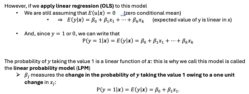
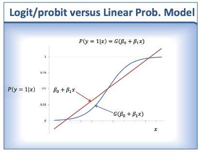
linear probability model (LPM)

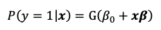
model where the probability of y (dummy) taking the value 1 is a linear function of x

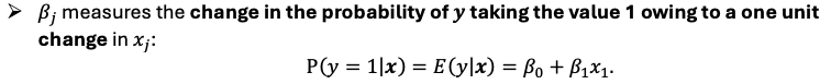
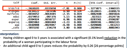
Interpreting the results from OLS after using for LDV

shows the gain / reduction on the probability of y = 1 (y is a dummy)

Dont bother looking at R²

How is goodness of fit measured for LPM (R² not used)

goodness of fit is measured by the percent of within-sample predictions that are “correct”

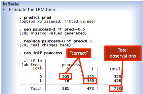
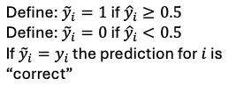
Goodnes of fit = (203+350) / 753 = 0.734

Heteroscedasticity and LPM

The variance of the error term depends on x → heteroscedasticity

•The estimated coefficients are unbiased and consistent but our inferences may be wrong owing to biases in the estimated standard errors

• Work using simulations suggests that these biases in the s.e.s are rarely large

• In Stata we can adjust s.e.s for heteroskedasticity and so in reality this isn’t usually a problem

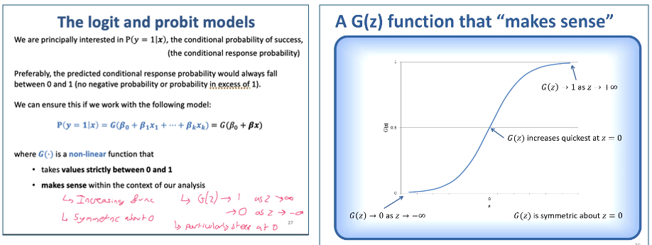
Why we use probit / logit models

Preferable we want the predicted conditional response to always fall between 0-1 (no negatives or greater than 1)

We enusre it using a non linear function

Logit / probit vs LPM

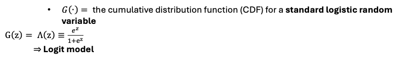
Logit model

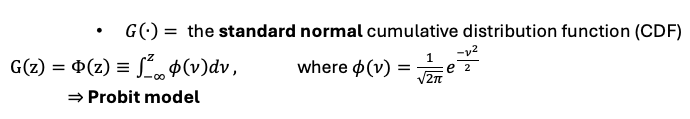
Probit model

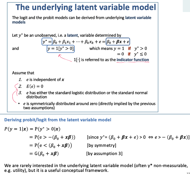
Deriving Logit / Probit models from underlying latent variable models

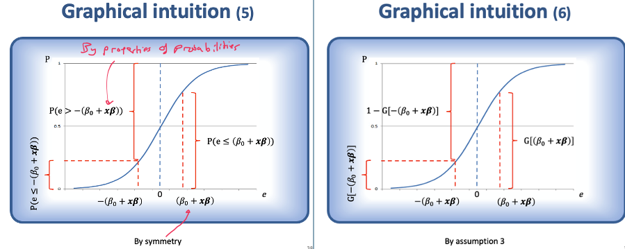
Graphical representation of probabilities and logit / probit models

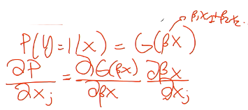
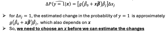
Why y (our dependent variable) is a function of x_j

We are interested in the effects of changes in the explanatory variables, x_j , on the conditional response probability

the latent variable y* is a linear function of x_j

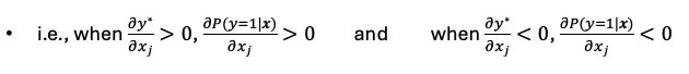
y is a non linear function of y* so is also nonlinear of x_j

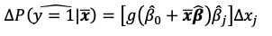
Effect of ∆x_j on prob of y = 1

G is a monotonically increasing function → anything that causes y* to increase also causes p(y = 1)

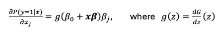
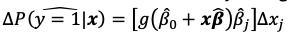
The marginal effect or partial effect of a continuous variable x_j on the probability of y = 1

given by the partial derivative of our probit or logit model with respect to x_j (same as in linear models)

Magnitude of marginal effect

depends on all the x’s we evaluate at

because g(z) > 0 for all z, the marginal effect always has the same sign as β_j

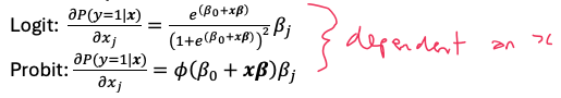
Marginal effect of a continuous variable on LPM

Marginal effect of a continuous variable on Logit / probit model

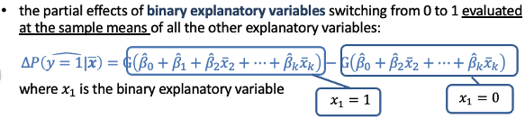
Binary X’s - effect of switching from 0→1

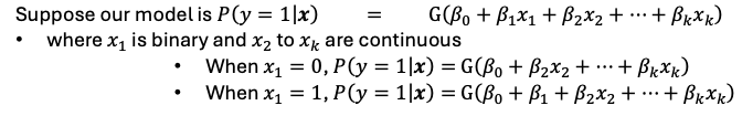
Depends on the values of x₂ , x₃ , etc

What to report with linear and non linear models

Usually, one reports:

•       the marginal effects of the continuous explanatory variables evaluated at the means of all the explanatory variables

•       the partial effects of binary explanatory variables switching from 0 to 1 evaluated at the means of all the other explanatory variables

When its a LPM it doesn't matter where you start - The marginal effect is always constant and does not depend on x.

While if non-linear function then it matters where we start as the change between values varies and isn’t constant

Can we use OLS for nonlinear models?

No we need to use maximum likelihood estimation (MLE)

maximum likelihood estimation (MLE)

Find the values of the β_j that maximize the likelihood of the observed y_i for our sample, given the x for our sample

Max the probability that our observed x's and y's come from that model

We maximize the sum of the log-likelihoods, L

L ≤ 0 because likelihoods are always between 0 and 1 so their logs are always negative

Logit / Probit estimators

No formula unlike OLS

Consistent (unbiased when n is large) + asymptotically normal + account for heteroscedasticity + asymptotically efficient

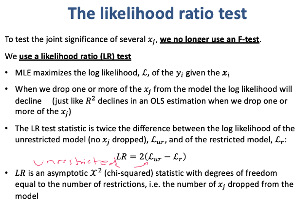
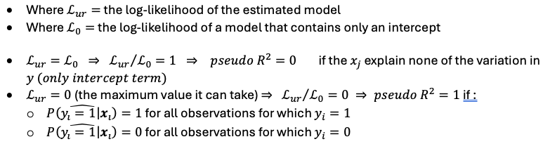
Likelihood ratio test

a measure of how MLE likelihood changes when we drop the x’s

Goodness of fit for MLE - percent correctly predicted

We can use “percent of observations correctly predicted” as our goodness of fit measure (just like for the LPM)

Goodness of fit for MLE options

• Percent correctly predicted

  • Pseudo R²

Goodness of fit for MLE - pseudo R²

R² = 1 - L_ur / L₀

Interpreting logit / probit estimates - Sign

The sign of an estimated coefficient indicates the sign of the marginal or partial effect of a change in the corresponding variable

• Can interpret it as usual

Interpreting logit / probit estimates - Significance

^β_j / se(^β_j) = z stat

An estimated coefficient, ^β_j divided by its standard error yields the z-statistic corresponding to the null hypothesis that x_j has no effect on y

• Just like for OLS, can interpret it as usual (like t statistic)

Interpreting logit / probit estimates - Magnitude

• The partial or marginal effects depend on x

• The same is true of estimated effect of any change in an x_j

Default option : reporting - Marginal effects

The marginal effects of the continuous explanatory variables evaluated at the sample means of all the explanatory variables

Why the default option is to report

The magnitude of our probit / logit estimators shows effect of changes of x_j on y

But x isnt defined so we need to choose an x before estimating the changes

We find the effects by using the sample means of all the explanatory variables

Partial (or marginal) effects at the average (PEA)

The estimates marginal / partial effects the for the sample average individual

We take a fictional individual that has the same characteristics as the average of all of the explanatory variables, and we are basically computing the marginal values for that person.

Average partial effects (APE)

the observed values of explanatory variables for individual i used to compute individual partial effect → then average across the sample