Ch 9 Notes Introduction to Keynesian Model

Notes from Class

Keynesian Model Characteristics

Very active role of government

Recession results from inadequate AD

Shirt-run view of the economy

Equilibrium may not equal full employment

Prices, wages & interest rates may be inflexible

Aggregate Spending (Expenditures)

C + I + G + NX

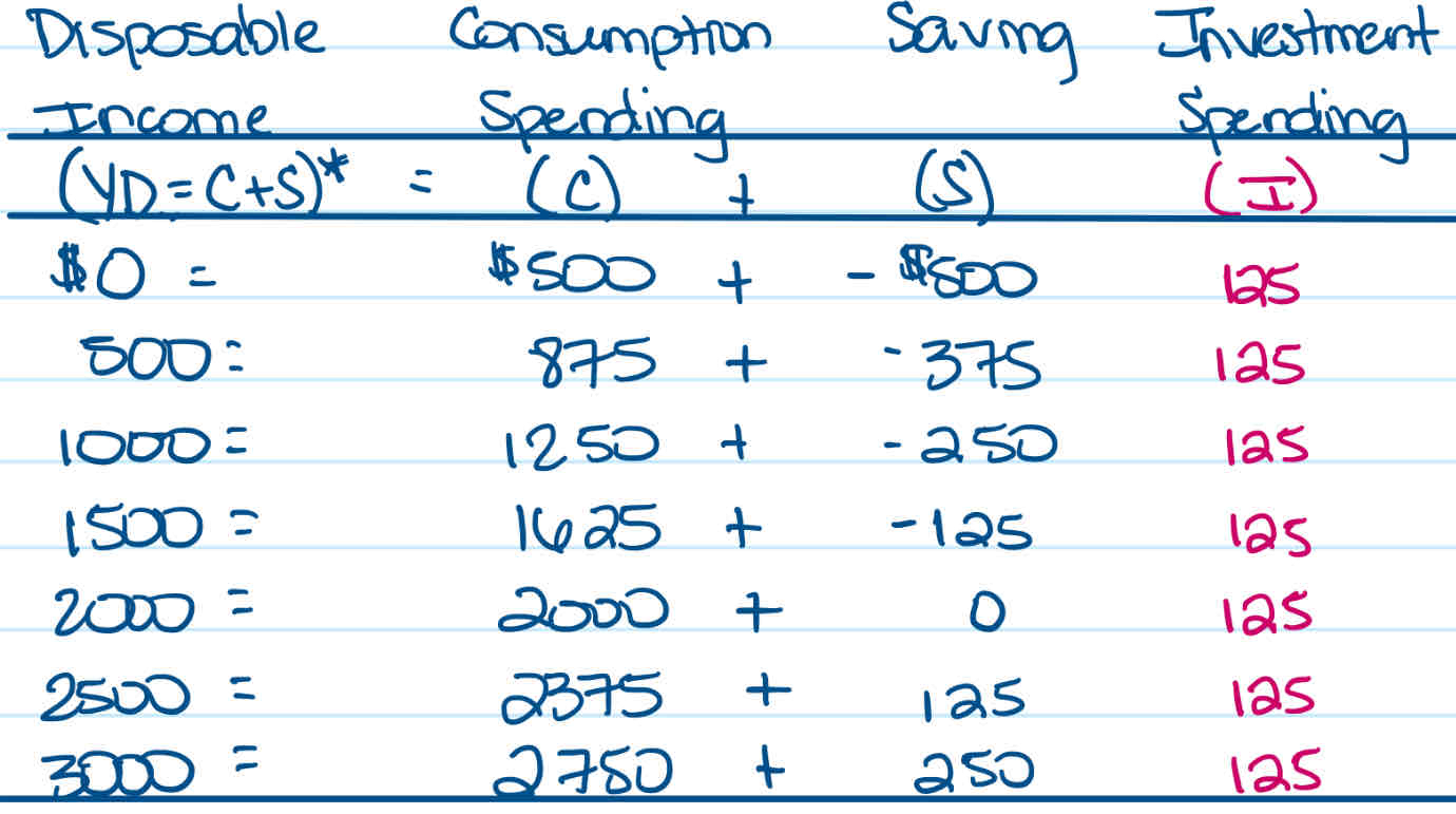
Consumption Spending Table

Propensities

Marginal Propensity to Consume (MPC)

Marginal Propensity to Save (MPS)

Marginal Propensity to Consume (MPC)

The change in (C) consumer spending associated with a change in (Yd) disposable income

MPC Formula

∆C = C2 - C1

∆Yd = Yd2 - Yd1

Marginal Propensity to Save (MPS)

The change in (S) saving associated with a change in (Yd) disposable income

MPS Forumla

∆S = S2 - S1

∆Yd = Yd2 - Yd1

Consumption Function

Shows the mathematical relationship between (C) consumption spending and (Yd) disposable income

General Expression of Consumption Function

C = Co + (MPC)(Yd)

Co in consumption function (C = Co + (MPC)(Yd) is

Autonomous Consumption

Autonomous Consumption

Amount of (C) consumption spending when (Yd) disposable income is 0

Break-even Income

The level of (Yd) disposable income when (S) Saving is 0

Investment Spending

Changes in the nations capital stock

(machinery, equipment, building, business spending)

Determinants of Investment Spending

Interest rate

Expectations of future sales, profits

Corporate taxes

Interest rates

Negatively related: When interest rates rise, the cost of borrowing increases, discouraging investment. Conversely, when interest rate fall, borrowing costs decrease, encouraging investment.

Expectations of future sales

Positively related: When businesses anticipate higher future sales and profits, they tend to increase investment spending to capitalize on these expected gains.

Corporate Taxes

Negatively Related: If taxes are raised, firms have less to spend and invest. Conversely, when taxes are lowered, firms have more to spend and invest.

Investment spending is assumed autonomous means

It is independent of changes in income or output levels. It's determined by factors like business expectations, technology, or government policies

Equilibrium Income

Closed economy

Private economy

Closed economy

No trade going on; no exports, no imports

Private economy

No government spending, no taxes

3 ways to determine equilibrium income

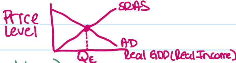
AD = AS (approach w/ graph)

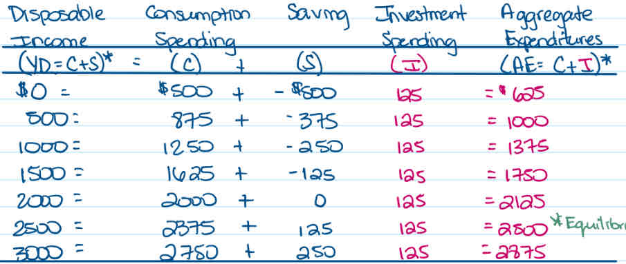
Saving = Investment (approach w/ table)

Aggregate Spending = Total Production (approach w/ formula)

AD = AS (approach w/ graph)

The point where AD curve intersects AS curve represents the equilibrium level of income

Saving = Investment (approach w/ table)

The point where saving (S) equals investment (I) is the equilibrium income level

125 = 125, so equilibrium is 2500

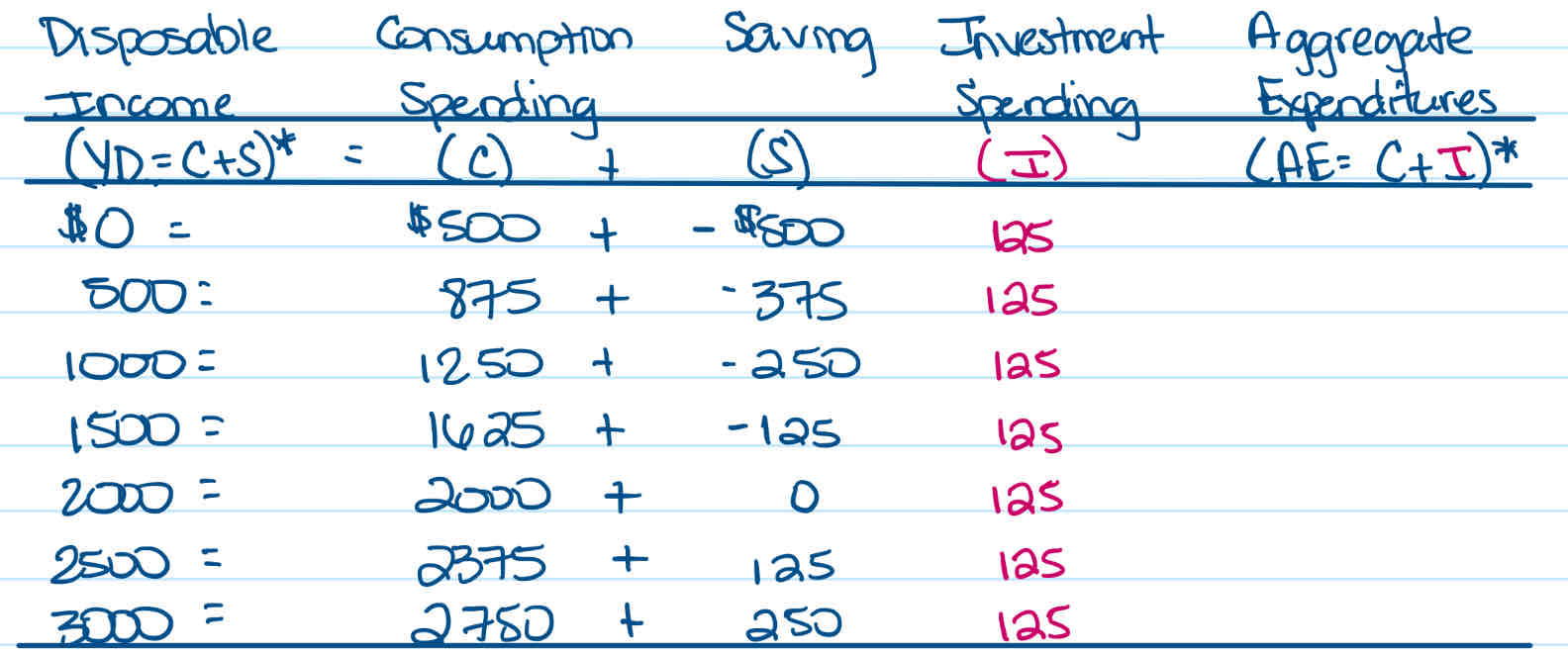
Aggregate Spending = Total Production

(In a closed economy, Aggregate Spending is just C + I, fill in table and find equilibrium income using consumption function formula)

Consumer Spending + Investment = Disposable Income

C + I = Yd

Co + (MPC)(Yd) + I = Yd

500 + .75(Yd) + 125 = Yd

625 + .75Yd = Yd

-.75Yd -.75Yd

625 = .25Yd

625/.25 = .25Yd/.25

2500 = Yd

Disequilibrium

Where AD ≠ AS. This can lead to unemployment or inflationary pressures.

Aggregate Spending < Total Production

(Demand < Supply = Surplus)

Inventories increase, production decrease, & unemployment increase

Aggregate Spending > Total Production

(Demand > Supply = Shortage)

Inventories decrease, production increase & unemployment decrease

Spending Multiplier

The multiple by which a small change in aggregate spending will result in a much larger change in real income (GDP)

Spending Multiplier Formula

1/1-MPC or 1/MPS

Aggregate Spending/ Real Income (GDP) Relationship

∆ Real Income (GDP) = (∆ Agg Spending) x (Spending Multiplier)

Adding (G) Government Spending & (T) Taxes - 3 sector model

Consumer Spending + Investment Spending + Government Spending = Total Production

C + I + G = Y

Solving for Equilibrium Income (GDP) in 3 sector model with given information:

(Y = income, Yd = disposable income = Y-T (income - taxes)

C = $200 + .80(Yd) I = $100 G = $200 T = $200

Aggregate Spending = Total Production

C + I + G = Y

$200 + .80(Yd) + $100 + $200 = Y

$200 + .80(Y-T) + $100 + $200 = Y

$200 + .80(Y-$200) + $100 + $200 = Y

$200 + .80Y - $160 + $100 + $200 = Y

$340 + .80Y = Y

-.80Y -.80Y

$340 = .20Y

$340/.20 = .20Y/.20

$1700 = Y

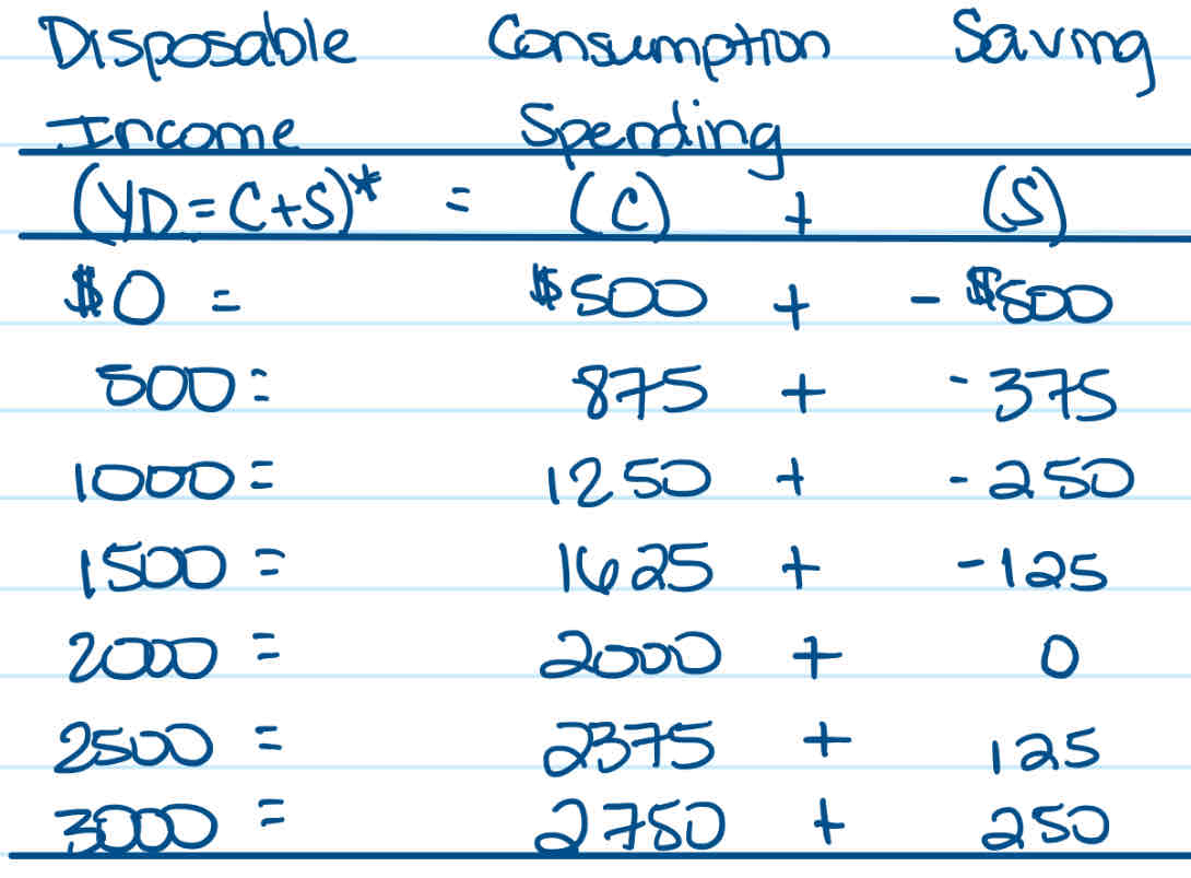
Use table to find MPC

MPC = ∆C/∆Yd

MPC = C2 - C1/Yd2 - Y1

MPC = 875 - 500/500 - 0

MPC = 375/500

MPC = .75

Use table to find MPS

MPS = ∆S/∆Yd

MPS = S2 - S1/Yd2 - Yd1

MPS = -375 - (-500)/500 - 0

MPS = 125/500

MPS = .25

MPC + MPS = 1

.75 + .25 = 1

Use the consumption function to find C when Yd is $1000. Verify with table.

C = Co + (MPC)(Yd) {*Co is amount of consumption spending when disposable income is 0}

C = 500 + .75×1000

C= 500 + 750

C = 1250

Use table to find break-even income

2000

Add Investment of 125 to table