VO 7+8+9 Data Assimilation

When was the first successful weather forecast?

Charney, Fjørtoft, von Neumann 1950

• computing time 24h for 24h forecast

Timeline weather forecast

• First operational numerical weather forecasts: → 1954 in Sweden
  → 1955 in the USA

  (although not really useful forecasts yet for several years)

• NWP pioneers HPC

• 1958: First generation of initial conditions using an objective analysis method at the National Meteorological Center (NMC; now the National Center for Environmental Prediction, NCEP)

• 1966: Primitive equations for NWP are used for the first time

• 1971: Creation of the first "nested" regional model

• 1978: The optimal interpolation (OI) technique is used for data assimilation for the first time → beginning of data assimilation, but initially limited to direct measurements of model variables

Evolution since 1980

• 1980: First spectral global model

• 1992: First ensemble forecasting system at ECMWF (but not really usable in

  the early years)

• From 1995: Development of "high-resolution" regional models, e.g., MM5 (USA), MC2 (Canada), Meso-NH (France), COSMO (formerly LM, Germany)

• 1996: ECMWF switches from the "optimal interpolation (OI)" technique for data assimilation to a 3-dimensional variational system (3D-Var) and one year later to 4D-Var (direct assimilation of satellite data/radiances)

• 2011: Introduction of "hybrid" data assimilation at ECMWF (use of an ensemble for error estimation). Other weather services switched around the same time or followed shortly after.

• 2012: Operational introduction of the DWD COSMO-DE ensembles as the first operational regional ensemble system

• 2023: First machine learning models in parallel operation

Why can raw NWP model output not always be directly used for local weather forecasts?

• Models cannot resolve local effects (zb ground inversion, local topography, fog, subgrid clouds)

• Models have systematic errors (zb precipitation intensity, ground temperature, cloud cover)

• Many different models and measurements (temperature, wind, radar) are available

• Model information is often several hours old by the time it reaches the user (computing time for data assimilation + model, transmission)

What is done during product generation and statistical post-processing?

• Calculation of additional diagnostic variables (sunshine, surface fields, cloud cover, model variables) from the prognostic model variables

• Mixing of different models (possibly weighting)

• Calculation of probabilities from ensembles

• Correction of model forecasts using current measurements

• Correction of systematic errors (Model Output Statistics, MOS), used in all automated forecasts

What is Model Output Statistics / MOS ?

→ Correction of systematic errors

• Over a training period (one year), the direct model output is compared with measurements (e.g., linear regression or machine learning)

• Different model fields and levels are linked (ground temperature errors can also depend on zb wind, inversion/stability, or fog/cloud cover)

• Automated corrections are then calculated for each location

• For certain variables (ground temperature), MOS is virtually unbeatable, but for rare extreme events, it sometimes struggles

27

What is blending in short-term weather forecasting and why is it used?

for short-term lead times (0-6h):

• combines nowcasting with NWP forecasts to improve forecast quality

Goal: create a smooth transition between the information sources using slowly changing weights.

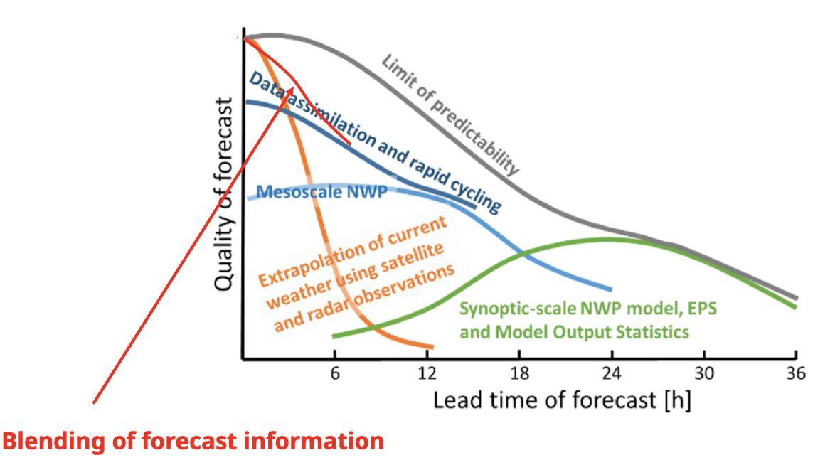
What is nowcasting, and why is it important at the beginning of the forecast period?

Nowcasting:

• extrapolation of current radar and satellite observations

• especially useful for the first 1–2 hours

• during this period, NWP forecasts are not yet available usually and sometimes produce artifacts (model spin-up)

What is Data Assimilation?

• Analysis = best estimate of the atmospheric state in the model space (model grid and model variables)

• If the problem is overdetermined:

  • more measurements than model degrees of freedom)→ averaging/interpolation

• problem is almost always underdetermined:

  • too few measurements

  • measurements unevenly distributed

  • measurements not equal to the model variable

• additional background information required:

  • climatology

  • rough estimate

  • persistence

  • short-term forecast

• In NWP: latest available forecast = background / first guess

• Mathematically optimal combination:

  • Least-squares method

  • Optimal weighting of measurements and background

Where else is data assimilation used?

• reanalysis

• oceanography

• medicine (MRI, CT, etc)

• Oil deposits

• astrophysics

• epidemic modeling

• animal populations

• etc.

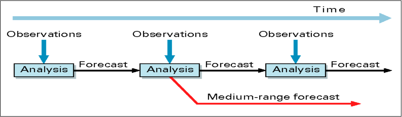
How does the ECMWF assimilation cycle work?

• observations are used to correct errors in the short-term forecast from the previous analysis time

• The analysis is mainly (> 95% information content) based on information from the short-range forecast, but this forecast also carries information from past observations into the current analysis
  → this means the information from observations is cycled

• The data assimilation procedure takes as much computer power as the 10-day forecast

• ECMWF has more staff working on data assimilation than on model development

  

What is the Gaussian distribution?

• 68% of values within ± σ (Standard deviation)

• 95% of values within ± 2σ

$$\sigma=\sqrt{\frac{\sum_{i=1}^{n}\left(x_{i}-\overline{x}\right)^2}{n-1}}$$

• Distribution that occurs frequently – and if not, a distribution can often be transformed to suit it

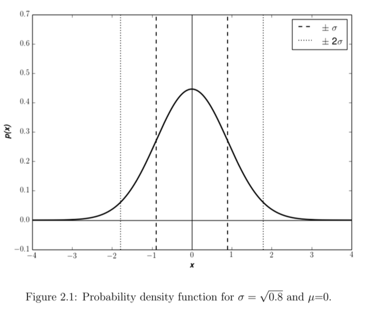
Properties of the Gaussian distribution?

• defined by two variables: mean and standard deviation (σ)

• Normal distribution remains normal under any linear transformation

Variables whose distribution and errors usually deviate from normal distribution:

• Humidity

• precipitation

• clouds/hydrometeors

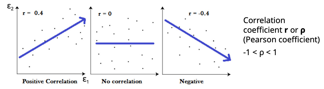
What does correlation between two errors ε1​ and ε2​ describe?

• Pearson correlation coefficient: −1 < r < 1

• r > 0: positive correlation

• r = 0: no linear correlation

• r < 0: negative correlation

• For uncorrelated errors:

$$\epsilon_1\cdot\epsilon_2=0$$

→ the expected value of the product of two errors is 0

• no causal relationship between the two errors

• Independent information from the two sources (information content is lower if

  errors are correlated)

Reality:

• Errors of model and measurement are usually uncorrelated

• Errors of different measurements are partially correlated

• Model errors are almost always spatially and temporally correlated (both an advantage and a disadvantage)

• The correlation coefficient describes only linear dependence; nonlinear relations, e.g. for clouds, may not be represented correctly

  

Easiest example for data assimilation

Given at a grid point:

• Measurement T_o (observation)

• Forecast T_b (background)

What we want:

• Optimal combination T_a (analysis) from T_o und T_b

• T_a should provide an optimal estimate of T_t (the truth)

Error epsilon:

$$\epsilon_{o}=T_{o}-T_{t}$$

$$\epsilon_{b}=T_{b}-T_{t}$$

$$\epsilon_{a}=T_{a}-T_{t}$$

Assumption:

• T_o and T_b have no systematic error (no bias): E(epsilon_o) = E(epsilon_b) = 0
  → where E() = expected value → average value over many realizations

• Mean errors of T_o and T_b are known and normally distributed: E(epsilon_o²) = epsilon_o^2 ; E(epsilon_b^2) = epsilon_b^2 → sigma = standard deviation → sigma^2 = variance

• Errors of To and Tb are not correlated: E (epsilon_o epsilon_b) = 0

BLUE - Best Linear Unbiased Estimate