ST411 Weeks 1-2: Introduction to Linear Regression

Outcome Y’s distribution

- $Y \sim f(y; \theta)$: $Y$ is a random variable that follows a probability distribution with pdf $f(\cdot)$ and parameter vector $\theta$ (vector or scalar).

- We often parametrize $\theta = (\mu, \psi)$, where:

- $\mu = \mathbb{E}(Y)$ is the expected value (mean),

- $\psi$ are zero or more additional parameters.

- The focus is typically on modeling the mean of the distribution ($\mu$).

How to think of regression modelling as specifications for conditional distributions (Y given X)?

$$Y \sim f(y| x \text{; } \theta)$$

Regression modeling provides a framework for defining conditional distributions of the response variable $Y$ based on predictor variables $X$.

It allows for estimating how the expected value of $Y$ changes with respect to variations in $X$ and the parameters $\theta$ of the conditional distribution.

Outcome Y’s distribution

- $Y \sim f(y; \theta)$: $Y$ is a random variable that follows a probability distribution with pdf $f(\cdot)$ and parameter vector $\theta$ (vector or scalar).

- We often parametrize $\theta = (\mu, \psi)$, where:

- $\mu = \mathbb{E}(Y)$ is the expected value (mean),

- $\psi$ are zero or more additional parameters.

- The focus is typically on modeling the mean of the distribution ($\mu$).

How to think of regression modelling as specifications for conditional distributions (Y given X)?

$$Y \sim f(y| x \text{; } \theta)$$

Regression modeling provides a framework for defining conditional distributions of the response variable $Y$ based on predictor variables $X$.

It allows for estimating how the expected value of $Y$ changes with respect to variations in $X$ and the parameters $\theta$ of the conditional distribution.

Models for the mean parameter $\mu$

Focus of this course, where the mean param $\mu$ of Y depends on X through a linear combination of the X’s.

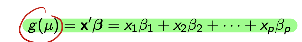
• g(.) is the link function where $g(\mu)=\mu$

• Beta’s are a vector of parameters - reg coeffs

How do we model the mean $\mu$ of $Y$ based on $x$?

The mean $\mu$ depends on $x$ through a linear combination:

  $g(\mu) = \mathbf{x}'\boldsymbol{\beta} = x_1 \beta_1 + x_2 \beta_2 + \cdots + x_p \beta_p$

What is $g(\mu)$?

- $g(\mu)$ is a link function, a specified function applied to the mean $\mu$ of $Y$.

- Example: In linear regression, $g(\mu) = \mu$ (identity link).

What is $\beta_0$?

- When the first element of $\mathbf{x}$ is 1, $\beta_0$ is the constant term or intercept in the model.

- $\mathbf{x} = (1, x_1, \ldots, x_{p-1})', \quad \boldsymbol{\beta} = (\beta_0, \beta_1, \ldots, \beta_{p-1})'$

What is the distribution of $Y$ in a standard linear regression model?

- $Y \sim N(\mathbf{x}'\boldsymbol{\beta}, \sigma^2)$

- The mean is a linear combination of explanatory variables.

- The variance $\sigma^2$ is constant (homoskedastic).

How does the expected value $\mu = \mathbb{E}(Y)$ depend on $\mathbf{x}$?

The mean is a linear combination, where the regression coeffs describe how the mean depends on each of the explanatory variables:

  $\mu = \mathbf{x}'\boldsymbol{\beta} = x_1 \beta_1 + x_2 \beta_2 + \cdots + x_p \beta_p$

What is assumed about the variance $\sigma^2$ in linear regression?

- The conditional variance $\sigma^2$ does not depend on $\mathbf{x}$.

- Variance is constant across all values of $\mathbf{x}$ (homoskedasticity).

What model do you use for continuous (normal) Y?

Linear regression

What model do you use for binary (binomial) Y?

Binary logistic regression

What model do you use for multinomial Y? (Provide distinction between nominal and ordinal model)

Nominal - multinomial logit model

Ordinal - cumulative (ordinal) logit model

What model do you use for Y where it is count data?

Poisson, negative binomial models, log linear models

What model do you use for duration Y?

Survival analysis models

What we need to understand for each model?

Linear reg. overview

• Is a GLM for a normally distributed Y and identity link

• Estimation done with maximum likelihood

• Inference using asymptotic results for ML estimation

Unique properties for linear regression

• MLE is also ordinary least squares estimation

• Normality → exact distributional results for test statistics and inference (as opposed to asymptotically)

• Model can also be motivated without distributional assumptions (using only mean and var. of Y)

What are the random variables and explanatory variables in the linear regression model?

• $Y_1, \dots, Y_n$ are independent random variables (responses).

• Each $Y_i$ has associated observed explanatory variables $\mathbf{x}_i = (x_{i1}, \dots, x_{ip})'$.

• $p \leq n$, and the $\mathbf{x}_i$ are treated as fixed.

Linear Regression Model: Distribution of $Y_i$

- What is the distribution of each $Y_i$?

• $$Y_i \sim N(\mu_i, \sigma^2)$$

• where $\mu_i = \mathbb{E}(Y_i) = \mathbf{x}_i' \boldsymbol{\beta} = x_{i1} \beta_1 + \cdots + x_{ip} \beta_p$.

• $\sigma^2$ is constant across all $i$ (homoskedastic).

Expected Value $\mathbb{E}(Y_i)$

- How is $\mathbb{E}(Y_i)$ expressed in terms of $\mathbf{x}_i$ and $\boldsymbol{\beta}$?

- $\mathbb{E}(Y_i) = \mu_i = \mathbf{x}_i' \boldsymbol{\beta} = x_{i1} \beta_1 + \cdots + x_{ip} \beta_p$

- A linear combination of explanatory variables.

Unknown Parameters in Linear Regression

- What are the unknown parameters in the linear regression model?

- The regression coefficients $\boldsymbol{\beta} = (\beta_1, \dots, \beta_p)'$.

- The residual variance $\sigma^2$.

Linear Regression Model: Matrix Form Setup

- How do we define $\mathbf{Y}$, $\boldsymbol{\mu}$, and $\mathbf{X}$ in matrix form?

* $\mathbf{Y} = (Y_1, \dots, Y_n)'$

* $\boldsymbol{\mu} = (\mu_1, \dots, \mu_n)'$

* $\mathbf{X} = [\mathbf{x}_1 \dots \mathbf{x}_n]'$ (an $n \times p$ matrix of explanatory variables)

Linear model in matrix Notation? Expression for $\mu$ ? And distribution.

$\mathbf{Y} = \mathbf{X}\boldsymbol{\beta} + \boldsymbol{\epsilon}$

$$\boldsymbol{\mu} = \mathbf{X}\boldsymbol{\beta}$$

* $\mathbf{Y} \sim N(\mathbf{X}\boldsymbol{\beta}, \sigma^2 \mathbf{I}_n)$

* $\mathbf{I}_n$ is the $n \times n$ identity matrix.

Definition as Mean + Residuals

- How can we rewrite the linear regression model using residuals?

* $\mathbf{Y} = \mathbf{X}\boldsymbol{\beta} + \boldsymbol{\epsilon}$

* where $\boldsymbol{\epsilon} = (\epsilon_1, \dots, \epsilon_n)' \sim N(0, \sigma^2 \mathbf{I}_n)$

- What are the properties of the residuals $\epsilon_i$?

* Each $\epsilon_i \sim N(0, \sigma^2)$

Residuals are *independent** of each other.

* All randomness in $\mathbf{Y}$ is attributed to $\boldsymbol{\epsilon}$.

• residuals are errors. They capture deviation of observed $Y_i$ from its mean $\mu_i = \mathbf{x}_i' \boldsymbol{\beta}$.

What assumption regarding residuals for linear regression?

$$\boldsymbol{\epsilon} \sim N(0, \sigma^2 \mathbf{I})$$

What does $\boldsymbol{\epsilon} \sim N(0, \sigma^2 \mathbf{I})$ imply? (4 items)

1. $\mathbb{E}(\epsilon_i) = 0$ for all $i$

2. $\text{var}(\epsilon_i) = \sigma^2$ for all $i$

3. $\epsilon_i$ and $\epsilon_j$ are independent for all $i \neq j$

4. Each $\epsilon_i$ is normally distributed

Estimation of $\boldsymbol{\beta}$: Method

- How is $\boldsymbol{\beta}$ estimated in linear regression?

• By Ordinary Least Squares (OLS)

• No distributional assumptions are needed (unlike Maximum Likelihood).

Ordinary Least Squares (OLS): Objective

- What is the goal of the OLS method?

Find $\boldsymbol{\beta}$ that minimizes the **sum of squared differences** between observed $y_i$ and expected $\mathbb{E}(Y_i \mid \mathbf{x}_i; \boldsymbol{\beta}) = \mathbf{x}_i' \boldsymbol{\beta}$.

Sum of Squared Errors: Formula

- What is the formula for the sum of squared errors in OLS? (equation and matrix notation)

$$S(\boldsymbol{\beta}) = \sum_{i=1}^n (y_i - \mathbf{x}_i' \boldsymbol{\beta})^2$$

Equivalently,

$S(\boldsymbol{\beta}) = (\mathbf{y} - \mathbf{X} \boldsymbol{\beta})'(\mathbf{y} - \mathbf{X} \boldsymbol{\beta})$

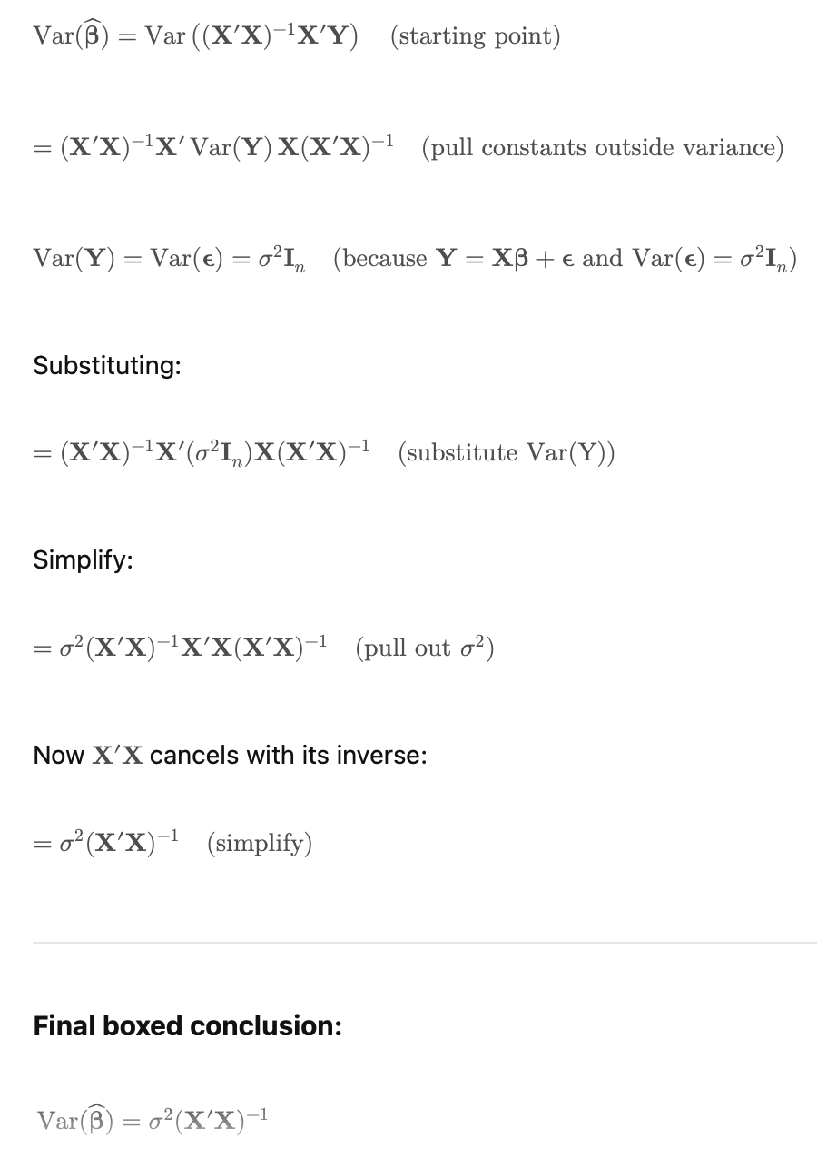
Definition of $\hat{\boldsymbol{\beta}}$

- What does $\hat{\boldsymbol{\beta}}$ represent?

* $\hat{\boldsymbol{\beta}} = (\hat{\beta}_1, \dots, \hat{\beta}_p)'$

* It is the value of $\boldsymbol{\beta}$ that minimizes $S(\boldsymbol{\beta})$ (the sum of squared errors).

OLS Estimator $\hat{\boldsymbol{\beta}}$: Derivation

- How is $\hat{\boldsymbol{\beta}}$ obtained?

* By solving:

  $\frac{\partial}{\partial \boldsymbol{\beta}} \left[ (\mathbf{y} - \mathbf{X}\boldsymbol{\beta})'(\mathbf{y} - \mathbf{X}\boldsymbol{\beta}) \right] = 0$

Involves taking a *partial derivative** and setting it to zero.

Full derivation of $\hat{\beta}$

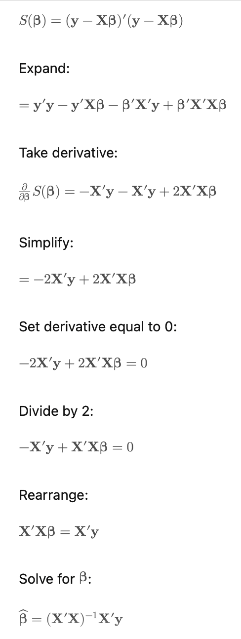
What is the final formula for $\hat{\boldsymbol{\beta}}$?

* $\hat{\boldsymbol{\beta}} = (\mathbf{X}'\mathbf{X})^{-1} \mathbf{X}'\mathbf{y}$

* Requires that $(\mathbf{X}'\mathbf{X})^{-1}$ exists (i.e., $\mathbf{X}'\mathbf{X}$ must be invertible).

Connection Between OLS and MLE

- When is the OLS estimator also the Maximum Likelihood Estimator (MLE)?

When the $Y_i$ are normally distributed

Under normality, OLS and MLE give the same estimate for $\boldsymbol{\beta}$

What is the formula for $\hat{\beta}_0$ in simple linear regression?

$$\hat{\beta}_0 = \bar{y} - \bar{x} \hat{\beta}_1$$

Estimator for Slope $\hat{\beta}_1$

- What is the formula for $\hat{\beta}_1$ in simple linear regression?

$\hat{\beta}_1 = \frac{\sum_i (y_i - \bar{y})(x_i - \bar{x})}{\sum_i (x_i - \bar{x})^2}$

This measures the scaled covariance between $x$ and $y$.

Alternative Expression for $\hat{\beta}_1$

- How else can $\hat{\beta}_1$ be written as a function of the sample standard deviation and correlations?

* $\hat{\beta}_1 = \left( \frac{s_y}{s_x} \right) r_{xy}$

* where:

  * $s_x$ = sample standard deviation of $x_i$

  * $s_y$ = sample standard deviation of $y_i$

  * $r_{xy}$ = sample correlation between $x_i$ and $y_i$

Unbiased Estimator of Variance $\sigma^2$

- What is the unbiased estimator for $\sigma^2$ in linear regression?

* $\hat{\sigma}^2 = \frac{1}{n - p} \sum_{i=1}^n (y_i - \mathbf{x}_i' \hat{\boldsymbol{\beta}})^2$

* Alternatively: $\hat{\sigma}^2 = \frac{1}{n - p} \mathbf{e}'\mathbf{e}$

* Divides by $n-p$ for unbiasedness.

Definition of Residuals

- How are the residuals $\mathbf{e}$ defined?

$$\mathbf{e} = \mathbf{y} - \mathbf{X}\hat{\boldsymbol{\beta}} = \mathbf{y} - \hat{\mathbf{y}}$$

-

Each residual: $e_i = y_i - \mathbf{x}_i' \hat{\boldsymbol{\beta}} = y_i - \hat{y}_i$

-

* e = vector of residuals (errors) for all observations

* y = vector of observed outcomes

* X = matrix of explanatory variables

* β̂ = vector of estimated regression coefficients

* ŷ = vector of predicted (fitted) values

* eᵢ = residual for the i-th observation

* yᵢ = observed outcome for the i-th observation

* xᵢ'β̂ = predicted value for the i-th observation (ŷᵢ)

* ŷᵢ = fitted value for the i-th observation

MLE Estimator of Variance $\sigma^2$

- What is the maximum likelihood estimator (MLE) of $\sigma^2$?

* $\hat{\sigma}^2_{ML} = \frac{\mathbf{e}'\mathbf{e}}{n}$

* Divides by $n$ (not $n-p$).

Formula for Residual Vector $\mathbf{e}$

- What is the formula for the residual vector $\mathbf{e}$?

* $\mathbf{e} = \mathbf{y} - \mathbf{X} \hat{\boldsymbol{\beta}}$

* Also written as: $\mathbf{e} = \mathbf{y} - \hat{\mathbf{y}}$ where y_hat is the fitted values

Formula for Individual Residual $e_i$

- What is the formula for the residual $e_i$?

* $e_i = y_i - \mathbf{x}_i' \hat{\boldsymbol{\beta}}$

* Also written as: $e_i = y_i - \hat{y}_i$

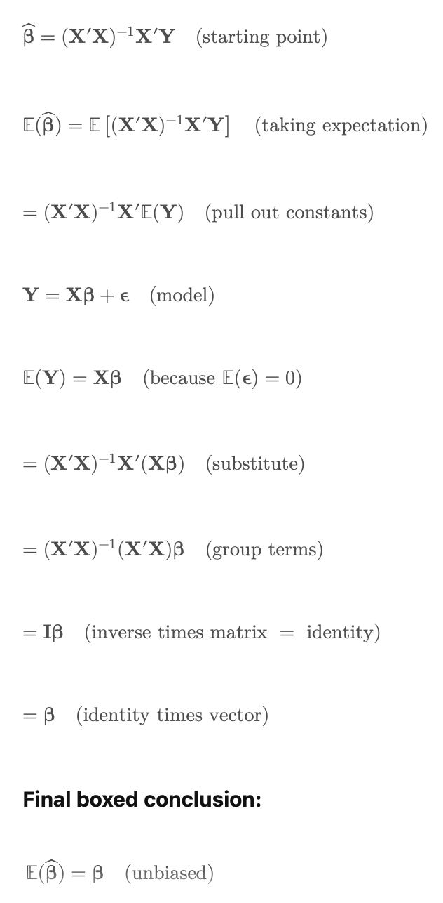
What is the expectation of $\hat{\boldsymbol{\beta}}$

$$\mathbb{E}(\hat{\boldsymbol{\beta}}) = \boldsymbol{\beta}$$

Thus, $\hat{\boldsymbol{\beta}}$ is an unbiased estimator of $\boldsymbol{\beta}$.

Derivation of $E(\hat{\beta})$

Variance of $\hat{\boldsymbol{\beta}}$

- What is the variance of $\hat{\boldsymbol{\beta}}$? (true variable of beta hat)

$$\text{Var}(\hat{\boldsymbol{\beta}}) = \sigma^2 (\mathbf{X}'\mathbf{X})^{-1}$$

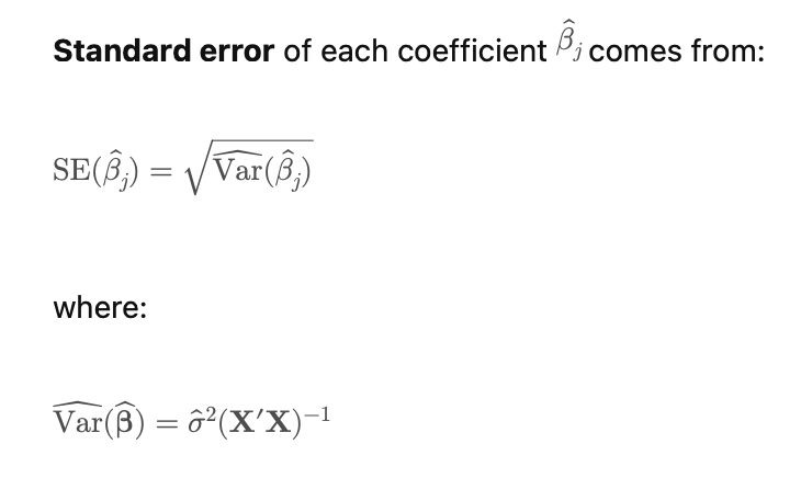
Unbiased Estimator of $\text{Var}(\hat{\boldsymbol{\beta}})$

- What is the unbiased estimator for $\text{Var}(\hat{\boldsymbol{\beta}})$? This is the estimated variance based on our data. We use sigma hat instead of sigma.

* $\widehat{\text{Var}}(\hat{\boldsymbol{\beta}}) = \hat{\sigma}^2 (\mathbf{X}'\mathbf{X})^{-1}$

* where $\hat{\sigma}^2$ is the unbiased estimator of $\sigma^2$.

* $\hat{\sigma}^2 = \frac{1}{n-p} \sum_{i=1}^n (y_i - \hat{y}_i)^2$

* $\hat{\sigma}^2 = \frac{1}{n-p} \mathbf{e}'\mathbf{e}$

* where $e_i = y_i - \hat{y}_i$ and $\mathbf{e} = (e_1, \dots, e_n)'$

Derivation of $\text{Var}(\hat{\boldsymbol{\beta}})$

Condition on $\mathbf{X}$ for OLS

- What condition must $\mathbf{X}$ satisfy for $\hat{\boldsymbol{\beta}}$ to be uniquely defined?

* $\mathbf{X}$ must be full rank: $\text{rank}(\mathbf{X}) = p$

* The inverse $(\mathbf{X}'\mathbf{X})^{-1}$ must exist.

* Condition fails if:

  * Columns are linearly dependent (multicollinearity)

  * or if $p > n$ (more variables than observations)

Distribution of $\hat{\beta}$

$$\hat{\boldsymbol{\beta}} \sim N\left(\boldsymbol{\beta}, \sigma^2 (\mathbf{X}'\mathbf{X})^{-1}\right)$$

$\hat{\boldsymbol{\beta}}$ is normally distributed because it is a linear combination of normally distributed $\mathbf{Y}$.

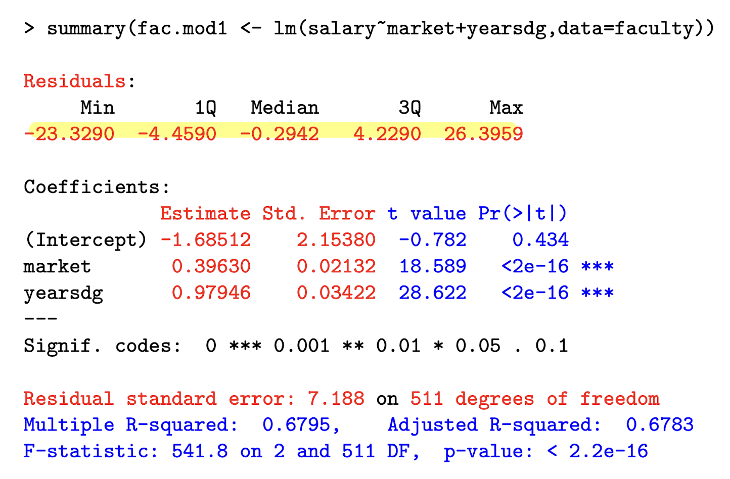
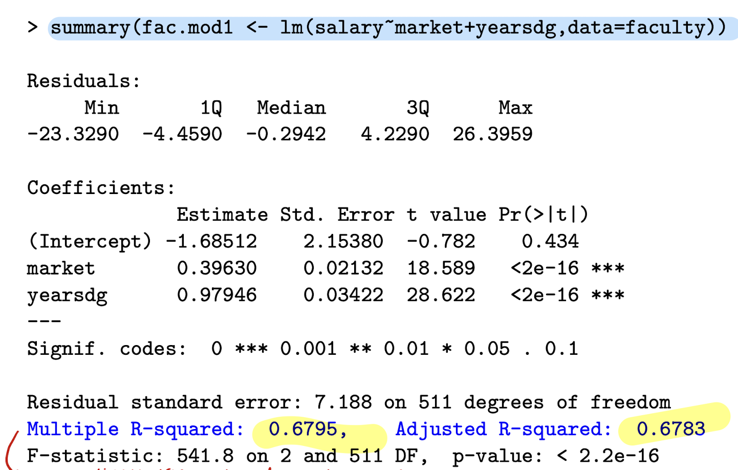
In R, how do you run a linear regression using faculty data, with response variable salary and explanatory vars market and yearsdg?

lm(salary ~ market + yearsdg, data = faculty)

Where can you find the distribution of residuals?

Label Beta_0, Beta_1, and Beta_2

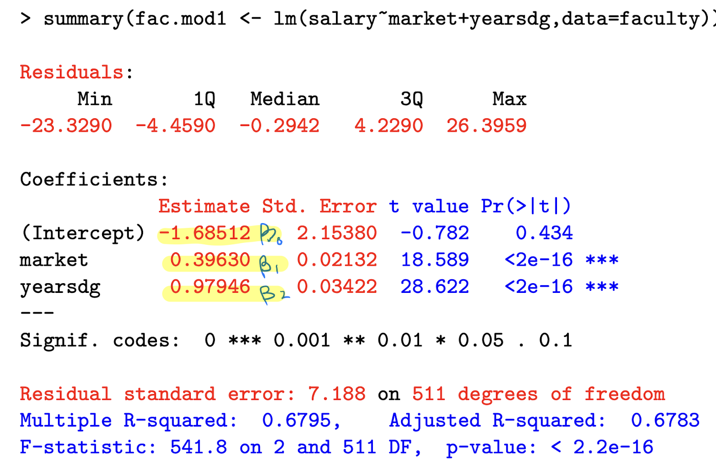
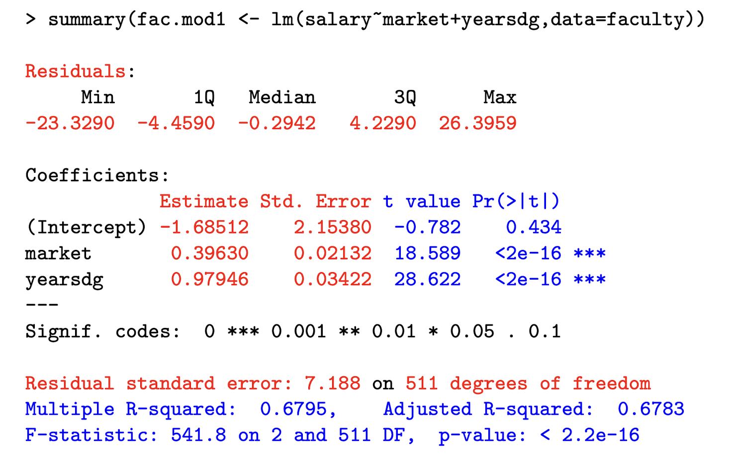
What is the “residual standard error” part telling you? How did it get 511 df?

It represents the square root of the unbiased estimate of $\sigma ²$, which we denote $\hat{\sigma}²$ .

$$\text{Residual standard error = } \sqrt{\hat{\sigma}²}$$

Where $\hat{\sigma²} = \frac{1}{n-p} e’e$

We get 511 df because we have 514 - 3 parameters (B0, B1, B2).

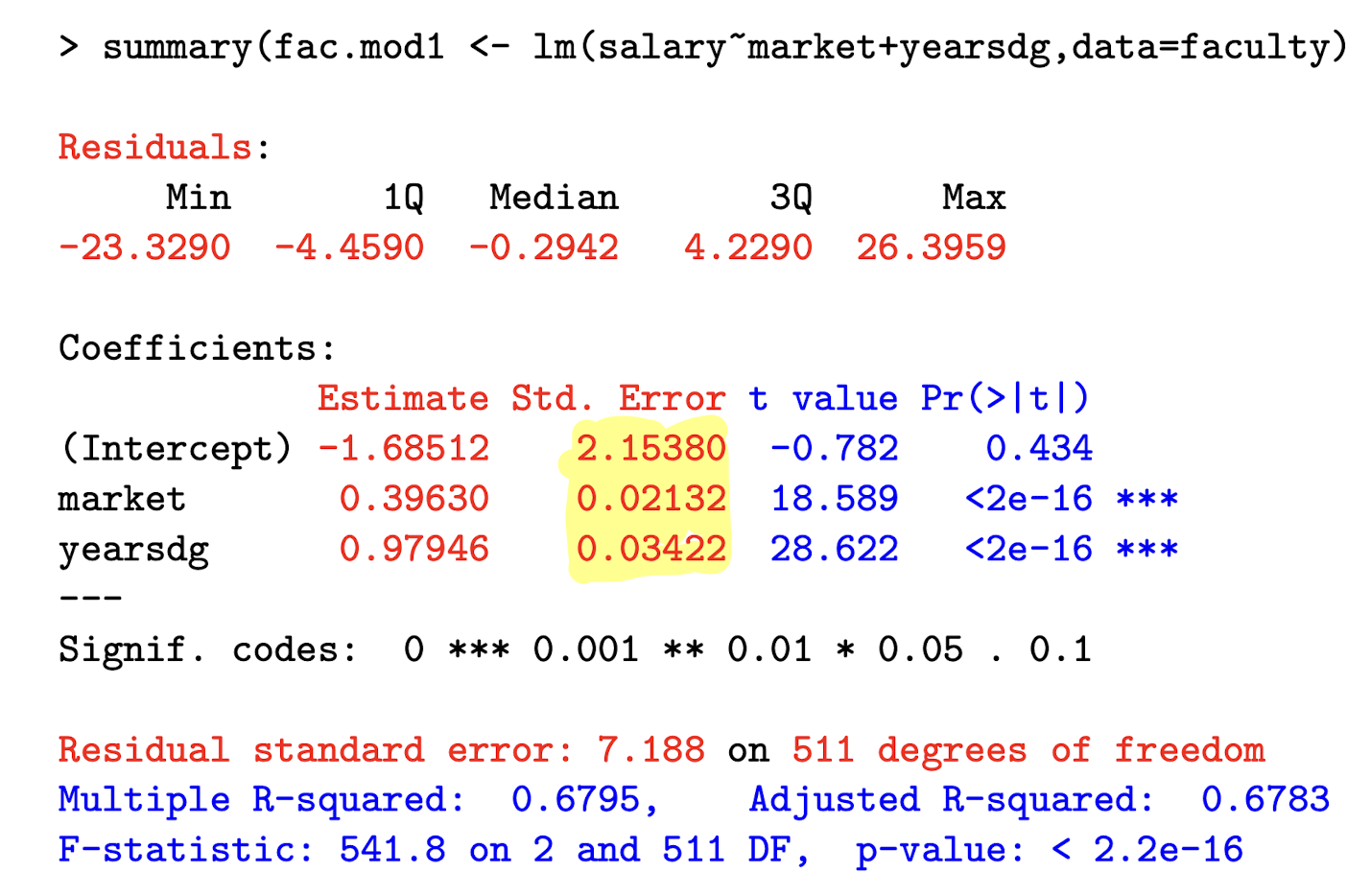
Explain how we get the standard errors for the betas?

General interpretation of regression coefficient on $x_j$ in a linear regression model

If $x_j$ increases by $a$ units, while controlling for other explanatory variables, the expected value of $Y$ changes by $a \cdot \beta_j$ units.

Interpret the coefficient on market , which the marketability point of their discipline. salary is in $1,000 units.

Holding other explanatory variables constant, a one-unit increase in the marketability of ones discipline increases the expected salary by $396 (0.396 × 1000).

What does TSS represent in regression?

* TSS = Total Sum of Squares

* $\text{TSS} = \sum_{i=1}^n (y_i - \bar{y})^2$

* Measures total variability in $y$ around its mean

* It’s the baseline variability before fitting any model

What is the decomposition of TSS in linear regression?

* $\text{TSS} = \text{XSS} + \text{RSS}$

* XSS = Explained (Regression) Sum of Squares

* RSS = Residual Sum of Squares

* This breaks total variation into model + leftover:

    * $\sum (y_i - \bar{y})^2 = \sum (\hat{y}_i - \bar{y})^2 + \sum (y_i - \hat{y}_i)^2$

What does XSS represent?

* XSS = $\sum (\hat{y}_i - \bar{y})^2$  

  * Measures improvement from using predictors  

  * Variation explained by the model (fitted values)

• Amount of the variation explained when the fitted values are allowed to depend on $x_i$ and thus vary by i.

What does RSS represent?

* RSS = $\sum (y_i - \hat{y}_i)^2$  

  * Measures how far the actual $y_i$ are from the model’s predictions  

  * Unexplained variation = residuals

What does TSS represent?

Describes the total variation in the values of $y_i$ in the sample.

What is the formula for $R^2$ (coefficient of determination)?

* $R^2 = \frac{\text{XSS}}{\text{TSS}} = 1 - \frac{\text{RSS}}{\text{TSS}}$

* Measures goodness of fit

* Tells how much of the total variation in $y$ is explained by the model

-

$R^2$ is the proportion of total variation in $y$ that is explained by variation in the explanatory variables.

* $R^2 \in [0, 1]$

* Closer to 1 → better model fit

How else can $R^2$ be calculated?

* $R^2 = (\text{cor}(y, \hat{y}))^2$

* It’s the square of the correlation between observed and predicted $y$ values

Interpret the R²

Interpretation example: $R^2 = 0.6795$

About 68% of the variation in salaries in this sample is accounted for by variation in years since PhD and marketability.

What is the formula for the adjusted $R^2$ statistic?

$$R^2_{\text{adj}} = \frac{(n - 1)R^2 - (p - 1)}{n - p}$$

How is adjusted $R^2$ different from regular $R^2$?

Adjusted $R^2$ does not necessarily increase when we add new explanatory variables

-

It accounts for model complexity using a penalty factor

-

It is more similar to penalised model assessment criteria such as AIC

What general form do most hypothesis tests in regression take?

$$\mathbf{R\beta = r}$$

$\mathbf{R}$ is a known matrix and $\mathbf{r}$ is a known vector — together they define constraints on $\boldsymbol{\beta}$

What is a null hypothesis for testing a single coefficient?

$$H_0: \beta_j = 0$$

Implies the coefficient of $x_j$ is 0, so $x_j$ can be omitted without loss

What is a hypothesis involving a linear combination of coefficients?

$$H_0: \beta_1 = \beta_2$$

Matrix form: $\mathbf{R} = [0\ 1\ -1]$ (B0, B1, B2) and $\mathbf{r} = 0$ .

More generally, that some coeffs are equal to each other.

What is an example of multiple simultaneous coefficient tests?

$H_0: \beta_1 = 0$ and $\beta_2 = 0$

$\mathbf{R} = \begin{bmatrix}0 & 1 & 0 \\ 0 & 0 & 1\end{bmatrix}$ and $\mathbf{r} = \begin{bmatrix}0 \\ 0\end{bmatrix}$

What is the sampling distribution of $\hat{\boldsymbol{\beta}}$ in normal linear regression?

$$\hat{\boldsymbol{\beta}} \sim \mathcal{N}(\boldsymbol{\beta}, \sigma^2 (\mathbf{X}'\mathbf{X})^{-1})$$

The estimated coefficients follow a normal distribution with mean equal to the true coefficients and a variance that depends on the error variance and the design matrix.

How do you compute $\text{se}(\hat{\beta}_j)$?

$$\text{se}(\hat{\beta}_j) = \sqrt{\sigma^2 \left[(\mathbf{X}'\mathbf{X})^{-1}\right]_{jj}}$$

Formula for t-statistic (general)?

$$t = \frac{\hat{\beta}_j - \beta_j}{\text{se}(\hat{\beta}_j)}$$

What is the formula for the t-statistic used to test $H_0: \beta_j = r$ or 0?

$$t = \frac{\hat{\beta}_j - r}{\text{se}(\hat{\beta}_j)} \sim t_{n - p} \quad \text{if } H_0 \text{ is true}$$

What distribution does the test statistic follow under the null?

It follows a $t_{n - p}$ distribution

What happens to the t-distribution if $n$ is moderately large?

It can be approximated by a standard normal distribution $\mathcal{N}(0, 1)$

What is the formula for a $(1 - \alpha) \times 100\%$ confidence interval for $\beta_j$?

$\hat{\beta}_j \pm t_{n - p}^{(1 - \alpha/2)} \cdot \hat{se}(\hat{\beta}_j)$

What does $t_{n - p}^{(1 - \alpha/2)}$ represent?

It is the $1 - \alpha/2$ quantile of the $t_{n - p}$ distribution used to determine the critical value for constructing confidence intervals.

What is the value of $t_{n - p}^{(0.975)}$ for a 95% confidence interval?

For large $n$, it approximates 1.96 from $\mathcal{N}(0, 1)$ .

In particular, for a 95% CI, $\alpha = 0.95$ .

What is the null hypothesis tested using $\mathbf{R\beta = r}$ when $\mathbf{R}$ is a $1 \times p$ row vector?

It tests a single linear constraint on $\boldsymbol{\beta}$, like $\beta_j = \beta_k$

What is the distribution of $\mathbf{R\hat{\beta} - r}$ under $H_0$?

$$\mathbf{R\hat{\beta} - r} \sim \mathcal{N}(0, \sigma^2 \mathbf{R(X'X)}^{-1}\mathbf{R'})$$

What is the formula for the t-statistic for testing $\mathbf{R\beta = r}$?

$$t = \frac{\mathbf{R\hat{\beta} - r}}{\sqrt{\hat{\sigma}^2 \mathbf{R(X'X)}^{-1}\mathbf{R'}}} \sim t_{n - p}$$

What is the key idea behind using matrix notation $\mathbf{R\beta = r}$ for hypothesis testing?

It allows us to test any single linear constraint on $\boldsymbol{\beta}$ — regardless of how many coefficients are involved — using a t-test

What kind of hypothesis does the F-test handle that the t-test cannot?

The F-test is used to jointly test multiple constraints — i.e., $q > 1$ constraints on $\boldsymbol{\beta}$

What does the null hypothesis $H_0: \mathbf{R\beta = r}$ look like in an F-test?

$\mathbf{R}$ is a $q \times p$ matrix and $\mathbf{r}$ is a $q \times 1$ vector, with $q > 1$ indicating multiple linear constraints on the coefficients.

What is the distribution of $\mathbf{R\hat{\beta} - r}$ under $H_0$?

$$\mathbf{R\hat{\beta} - r} \sim \mathcal{N}(0, \sigma^2 \mathbf{R(X'X)}^{-1} \mathbf{R'})$$

What is the formula for the F-statistic used in this test?

$$F = \frac{(\mathbf{R\hat{\beta} - r})' (\hat{\sigma}^2 \mathbf{R(X'X)}^{-1} \mathbf{R'})^{-1} (\mathbf{R\hat{\beta} - r})}{q} \sim F_{q, n - p}$$

How are the t-test and F-test related when $q = 1$?

$F = t^2$ and the tests give the same p-value since $F_{1, n - p} = t_{n - p}^2$

What is the big-picture idea of the F-test as a comparison of nested models?

The F-test can compare two nested models by testing whether a subset of regression coefficients are all zero — i.e., whether adding predictors significantly improves model fit

What is the null hypothesis in the nested model version of the F-test?

$H_0: \beta_j = 0$ for all $j \in S_j \subset \{1, \dots, p\}$ — i.e., a subset of coefficients are all zero.

How are Model 0 and Model 1 defined in a nested model comparison?

Model 0 is the restricted model under $H_0$ with predictors ($x_1, x_2$), the model under the null.

Model 1 is the full model under $H_1$ ($x_1, x_2, x_3, x_4$) , the model under the alternative.

Model 0 is obtained from Model 1 by setting $\beta_3 = \beta_4 = 0$, so Model 0 is nested in model 1.

What is the general null hypothesis when comparing nested models by F-test?

If Model 0 has $p_0$ predictors and Model 1 has $p_1$ predictors where p1 > p0.

$\beta_*$ are the predictors in $\beta_1$ but not in $\beta_0$.

$$H_0: \beta_* = 0 \text{ (Model 0)}$$

$$H_1: \text{At least one of the coefficients is non-zero}$$

What is the F-statistic formula using residual sums of squares (RSS)?

$$F = \frac{(RSS_0 - RSS_1)/(p_1 - p_0)}{RSS_1 / (n - p_1)} \sim F_{p_1 - p_0,\, n - p_1}$$

$$F = \frac{(R_1^2 - R_0^2)/(p_1 - p_0)}{(1 - R_1^2)/(n - p_1)}$$

$$F = \frac{n - p_1}{p_1 - p_0} \cdot \frac{RSS_0 - RSS_1}{RSS_1}$$

What are the two formulations of the F-test, and how do they differ in logic?

1. The Wald (t-test) form tests whether $\hat{\boldsymbol{\beta}}_*$ are close to 0 relative to their variances

2. The nested model form tests whether Model 0 explains the data nearly as well as Model 1 (which includes $\boldsymbol{\beta}_*$).

Wald form ≈ Wald test

Nested model form ≈ Likelihood ratio test

IN LINEAR REGRESSION, THE WALD AND LR TEST VERSIONS OF THE F-TEST ARE EQUIVALENT. The Wald test evaluates the significance of individual coefficients, while the nested model form assesses overall model fit by comparing explanatory power between the two models.

What happens when the F-test has only one constraint ($q = 1$)?

It becomes a test of $H_0: \beta_j = 0$ and the F-statistic reduces to $F = t^2$ — the test is equivalent to the t-test

What is the null hypothesis in the F-test when $\boldsymbol{\beta}_*$ includes all coefficients except the intercept?

That all explanatory variable coefficients are zero — i.e., $H_0: \beta_1 = \dots = \beta_{p-1} = 0$

What is the F-statistic formula when testing if all explanatory variable coefficients are zero?

$$F = \frac{n - p}{p - 1} \cdot \frac{TSS - RSS}{RSS} = \frac{(R^2)/(p - 1)}{(1 - R^2)/(n - p)} \sim F_{p - 1,\, n - p}$$

where n is the sample size, and p is the number of parameters. In this case, RSS0 = TSS and R²_0 = 0.

This test is usually reported in standard reg. output, but not really an interesting hypothesis.

What are residuals, and why are they useful in regression diagnostics?

Residuals are $e_i = y_i - \mathbf{x}_i'\hat{\boldsymbol{\beta}}$.

They help check whether model assumptions are satisfied - To check model assumptions like normality, constant variance, correct specification, and influence of individual observations