Microeconomics S2

What is market structure?

market structure is the characteristics of a market that may influence behaviour and performance (their output and price)

Characteristics of a market

• the number and size of sellers

• barriers to entry

• extent of product differentiation

• number and size of buyers

2 rules for profit maximisation

1. SHUTDOWN RULE: The firm should shut down if price is less than Average variable cost (in short-run) or LRAC (long-run average costs where all factors are variable)

2. MARGINAL OUTPUT RULE: If the firm doesn’t shut down it should produce at the level where MR = MC

Assumptions of perfect competition

• buyers are price takers (can buy as much as they want without affecting price)

• sellers and buyers have complete information

• sellers are price takers (sellers output choice won’t impact price as wont trigger reaction from rivals due to low competitive behaviour → firms don’t actively compete with each other)

• entry is free AKA no barrier to entry and exit

Perfect competition market structure characteristics

• Many small number of sellers

• low barriers to entry and exit

• undifferentiated identical/ homogenous products (very unrealistic but closest to agricultural goods and primary commodities)

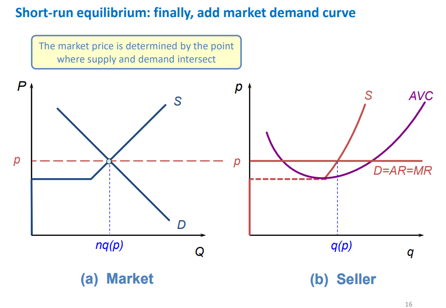
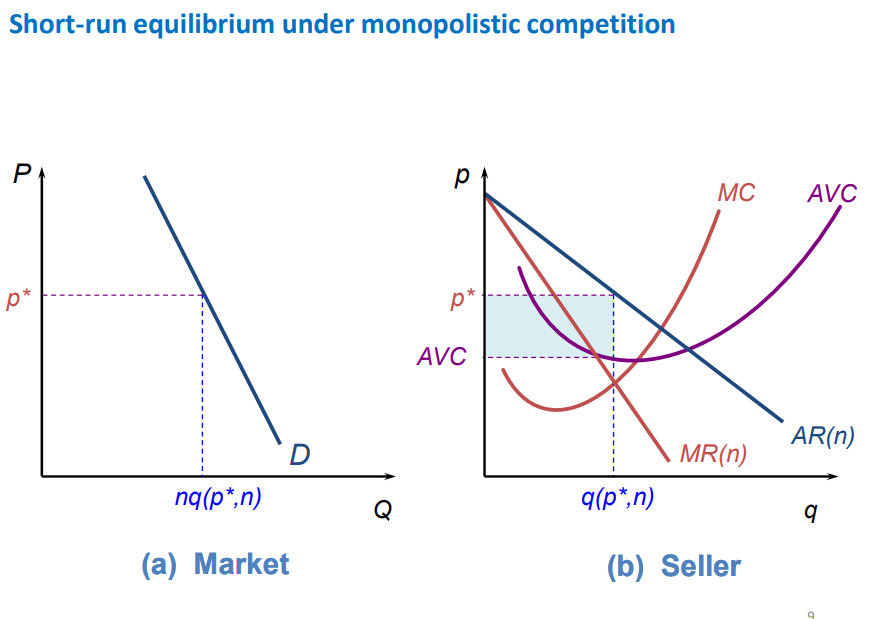
Perfect competition short-run equilibrium

when sellers produce as much as buyers want to purchase and buyers purchase as much as sellers choose to produce (

market price determined by where market supply and demand intersect (graph on left)

a sellers output is determined by seller-specific supply and demand (which is the specific MC and AVC on the right and output is when MC=MR) → profit max, may make supernormal profits, losses or break-even in short-run

supply falls off at min AVC as under this firms would shut down

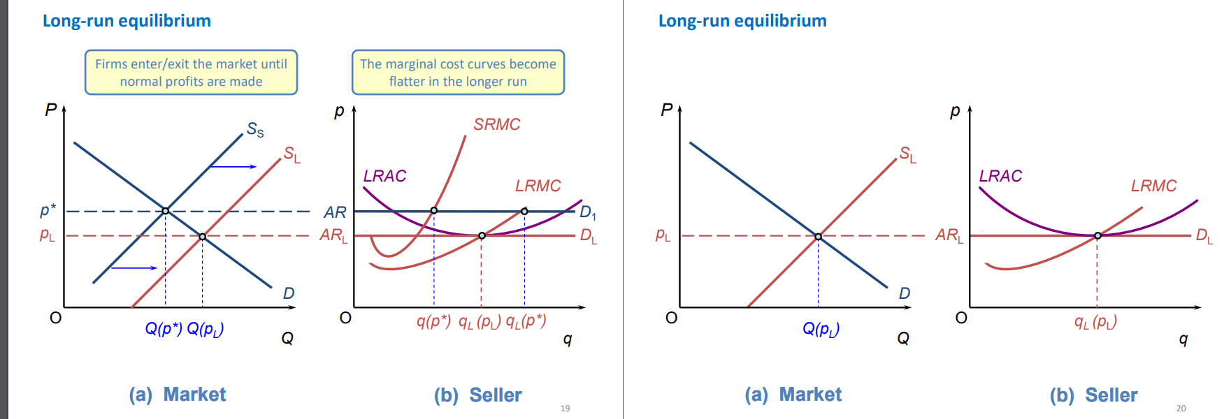
Long-run equilibrium perfect competition

equilibrium changes in long-run because:

• all factors are variable which impacts seller’s costs (LRAC is a flatter curve)

• sellers can freely enter and exit market (e.g. if making profits this attracts new sellers which increases market supply and reduces price)

= sellers make normal (zero) profit in the long-run where sellers in market are incentivised to stay and none are incentivised to enter (under assumption firms are profit seeking)

welfare maximised, socially efficient, productively efficient and allocatively efficient

declining industries

low revenues mean firm is unable to afford replacing old equipment with new ones so equipment begins wearing out.

HOWEVER people tend to blame an industry’s decline on this old equipment

so old equipment is often AN EFFECT rather than a cause of an industry’s decline

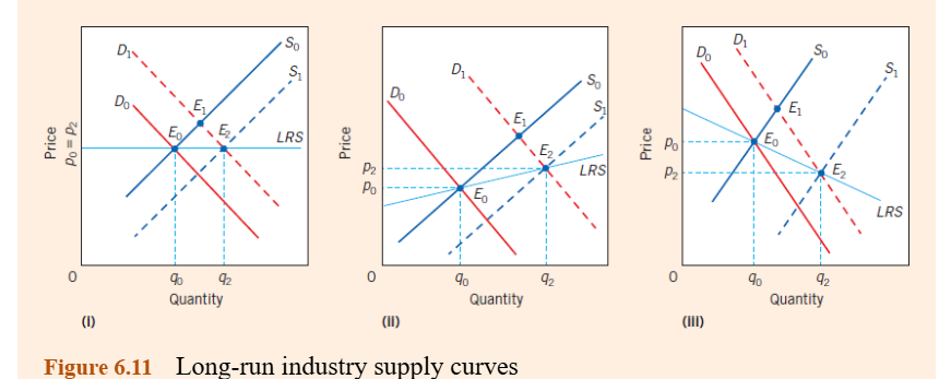
Long-run industry supply prices

in the long-run the industry supply curve ( may be:

• horizontal = constant cost industry occurs when input prices don’t change when output expands or falls

• rising/upwards sloping = when as as industry expands its output it needs more inputs and the increased demand for inputs raises their prices, as suppliers costs rises they raise their prices to cover their costs

• negatively sloped = when industries supplying their inputs have increasing returns to scale which reduce their prices = suppliers costs fall and may reduce their prices

Allocative efficiency of perfect compeitition

consumer and producer surplus is maximised so perfectly competitive markets allocate resoruces efficiently

monopoly

one dominant seller of a particular good or service, no competition

only producer in an industry so set market prices as firm = market

Monopoly assumptions

• the monopolist is a price maker (influences price by changing output → means demand curve is downwards sloping + no competition as large market power to change price)

• high barriers to entry (even in long-run potential sellers aren’t free to enter market → barriers may be legal requiring specific qualifications, structural e.g. by lowering AC by producing more so new firms who start by producing more can’t reap same profits, strategic behaviour to deter rivals

Monopoly market structure

One large seller

high barriers to entry

differentiated unique product

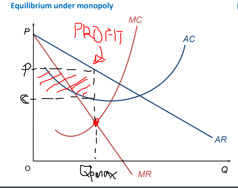
Monopoly equilibrium

determined by profit maximisation so where MR=MC

trace up to find cost on AC curve and price on AR curve

marginal revenue lies under AR

profits are sustained in the long-run and give incentive for research and development and finding new technologies

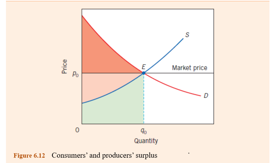
consumer and producer surplus

consumer surplus: the difference between the amount consumers are willing to pay and what they actually pay (difference between demand curve and price)

producer surplus: the difference between the price of a good and the minimum price producers are willing to supply it (difference between supply curve and price)

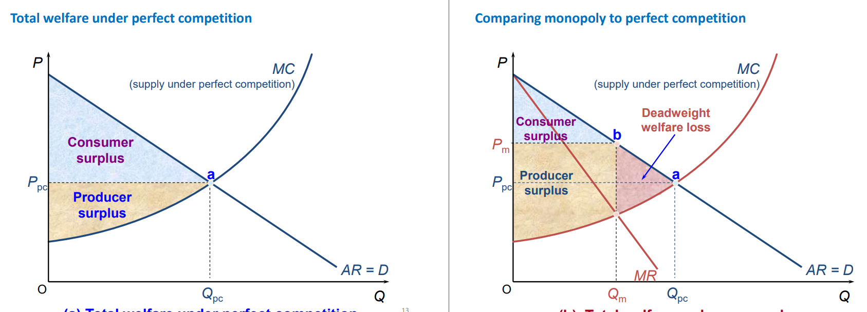
Comparing monopoly to perfect competition

total welfare (consumer + producer surplus) is greater under perfect competition than under monopoly

monopoly has welfare loss → creates rational case for government intervention to prevent formation of monopolies or control their behaviour

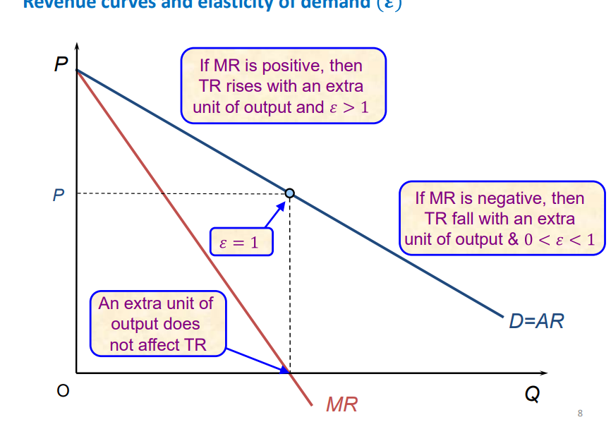
Revenue curves and elasticity

when marginal revenue = 0, elasticity of AR is 1 and TR is maximised → will always produce on elastic part of demand curve as want high revenue to maximise profits

when MR is positive, TR rises by more, so elasticity of AR is larger than 1

When MR is negative, TR falls so elasticity of AR is inelastic (between 0 and 1)

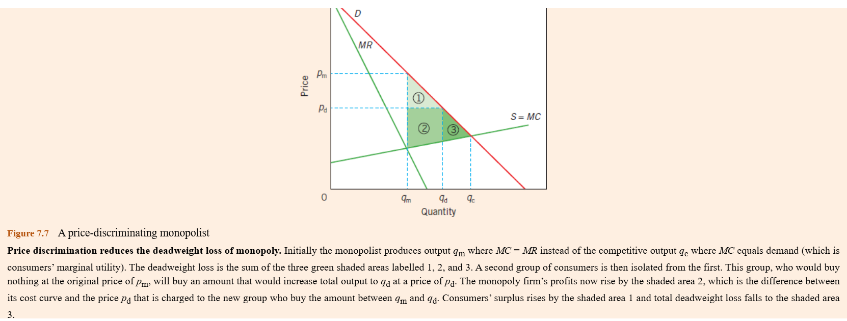
price discrimination

when a seller charges different prices for different units of the SAME product or service for reasons not associated with differences in cost

e.g. cinema tickets for children, students and adults, airline tickets on different dates

the ability to charge multiple prices (such as charging higher prices to those willing to pay more) gives the seller the ability to increase consumer surplus and decrease welfare loss

price discrimination allows firms to sell more without decreasing market price

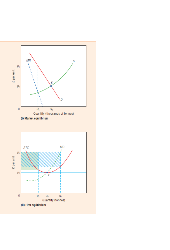
cartels

when firms in an industry agree to cooperate with one another and behave as a singe seller/monopoly to maximise joint profits by eliminating competition

e.g. agree to set quota on output so produce at Q1 instead of Q0 equilibrium, which maximises profits

problems cartels face

• ensuring all members follow behaviour that will maximise the industry’s joint profits (rather than succumbing to self interest)

• preventing the profits being eroded by the entry of new firms

price discrimination vs single price

price discrimination is more profitable and has no welfare loss

conditions necessary for profitable price discrimination?

1. sellers must be price makers → in order to set the different prices

2. buyers must differ and sellers must be able to identify the different buyers in order to discriminate prices

3. consumers must not be able to participate in arbitrage (when buyers charged a low price purchase the good and resell it e.g. students cant resell to non-students due to proof of student status needed)

Assumptions of price discrimination

• the seller is a pure monopolist (price discrimination can occur in markets with more than one seller but assume its a monopolist to understand problem without complications)

• entry is blocked even in long-run so analysis doesn’t change between short-run and long-run

Types of price discrimination and definitions

1. First degree price discrimination: when sellers charge each individual buyer the maximum price the buyer is willing pay

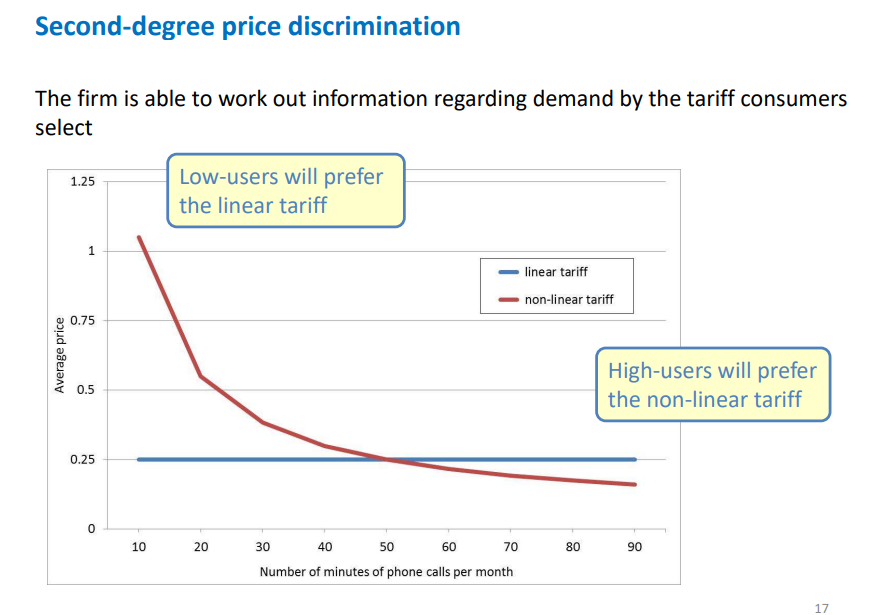
2. second degree price discrimination: a seller can use a menu of ‘non-linear tariffs’ (non-linear when average price changes) to get buyers to reveal their preferences when they select a tariff e.g. £10 per month vs 5p per minute for calls

3. third degree price discrimination: when a seller can identify groups of buyer and charge different prices to each group (can be grouped by characteristics such as students, or by location e.g. affluent areas charged more)

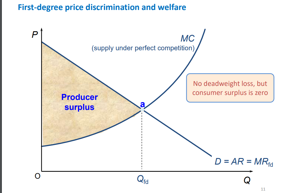
first degree price discrimination and diagram

Marginal revenue is equal to Average revenue (= price)

therefore there is no deadweight loss

produces same output as a perfectly competitive seller = more than what it would without price discrimination → more profitable

since every consumer is paying maximum there is no consumer surplus (no difference between what they pay and what they are willing to) so maximum welfare is fully producer surplus

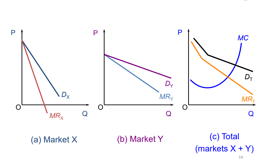
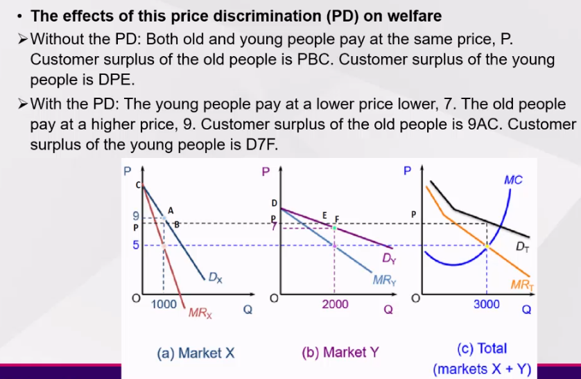
third degree price discrimination and diagram

different markets/groups have different elasticities

groups willing to pay more will have inelastic demand (market X) → benefit without price discrimination as offered lower prices to accommodate for elastic demand

groups not willing to pay as much will have elastic demand (market Y)

total market will add the market curves together horizontally so MC =MR on total market aligns with a point on MRy and MRx

produces same output as without price discrimination, deadweight loss as AR (D) is above MR

price charged in single price monopolist lies between the prices charged to the two groups

3rd degree price discrimination effect on welfare

increases welfare for the elastic group (price falls so consumer surplus increases)

decreases welfare for inelastic group price rises so consumer surplus falls)

there is deadweight loss as the price (AR) is not equal to MC

linear vs non-linear tariff

low users will prefer linear tariff

high-users will prefer non-linear tariff

forms of imperfect competition

monopolistic competition

oligopoly

2 ways products can be differentiated

• horizontal differentiation: same quality (so similar/same price) but choices depend on peoples tastes and preferences

• vertical differentiation: quality (and also price) clearly differs

Assumptions regarding monopolistic competition

• buyers are price takers

• buyers and sellers have complete information

• sellers are price MAKERS (so seller sells more when price is lower and their output choice isn’t reacted to by rivals)

• entry is free so potential sellers can enter market in the LONG run

Monopolistic competition market structure

• many small sellers

• low barriers to entry

• differentiated products either horizontal or vertical

Short run equilibrium monopolistic competition

price maker so downward sloping demand curve

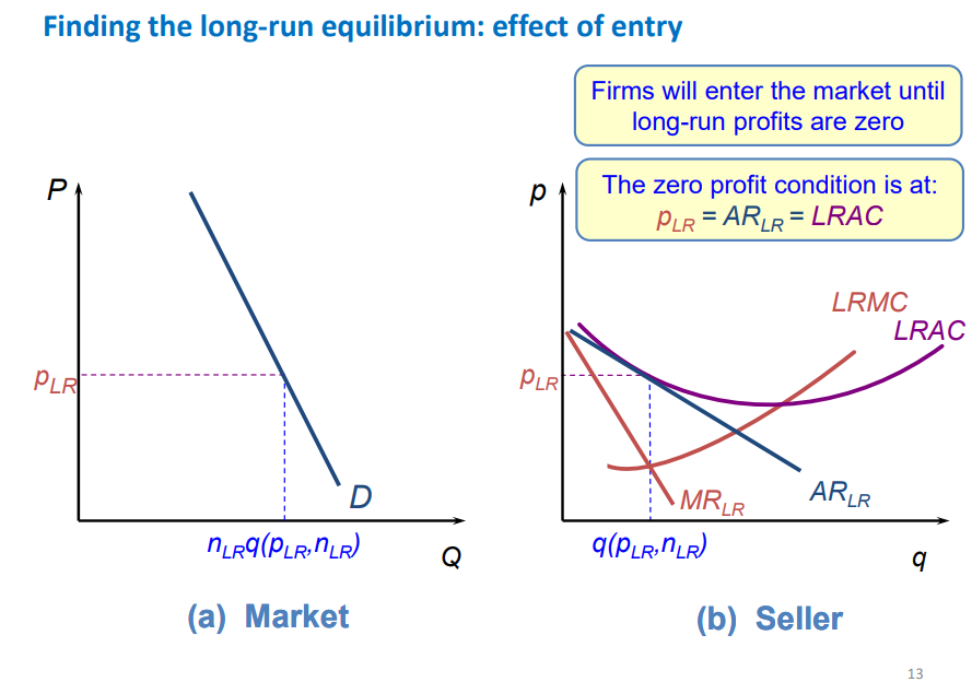
long run equilibrium monopolistic competition

in long run other sellers can freely enter the market and all factors are variable which impacts sellers costs

long-run costs curves LRAC and LRMC are flatter

make normal profit in long run as when firms enter the market (more sellers) this leads to lower demand for an individual seller as there are the same amount of buyers between a larger amount of sellers

differences between monopolistic competition and perfect competition

1. price-cost margin: in perfect competition price is always equal to marginal cost but in monopolistic competition price is above marginal cost

2. capacity: perfectly competitive sellers operate at FULL CAPACITY as they produce at the minimum efficient scale (lowest possible cost) no matter how much they produce whilst monopolistically competitive sellers have EXCESS CAPACITY as firms can produce more to lower their costs

game theory and terms definitions

used to highlight strategies to maximise gains/minimise losses

helps make predictions about how economic agents will behave in certain situations

players → decision makers aka sellers

strategies → pricing decisions

payoffs → how well players do e.g. profits

representation of games

1. extensive form = sequential move games where player A moves first then player B moves, game represented as a tree diagram

2. normal form = players move simultaneously, game represented by matric (more strategies (aka choices) = larger matrix 2×2, 3×3 etc.

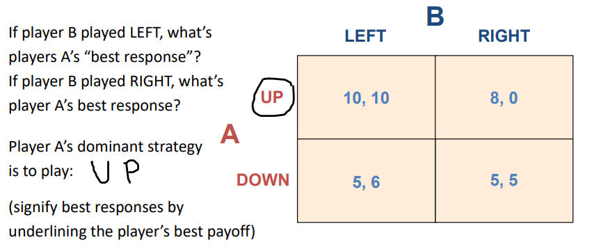
dominant strategy

a strategy is dominant if it provides a player with the highest payoffs regardless of a opponents strategy

can have dominant strategy equilibrium if both players dominant strategy (highest payoff) is at same point (here would be up left)

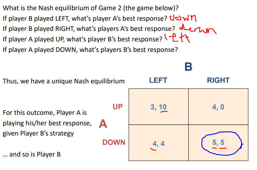
nash equilibrium

when no player can do better than their chosen strategy given their beliefs of how other players will play

two requirements:

1. each player must be playing a best response against their belief of how other players will play

2. these beliefs must be correct

(in image nash equilibrium where both are underlined as both players playing best response to others strategy)

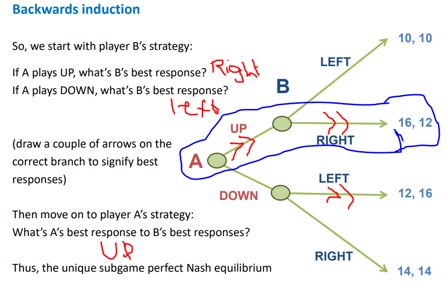
subgame perfection

refinement of nash equilibrium for sequential move games

split tree map into subgames (e.g. what B does if A chooses up)

use backwards induction in each subgames where you start at end of game to solve for best responses

put extra arrows at best choice, nash equilibrium when arrow goes from both A and B

models of oligopolies

quantity setting (Cournot)

price setting (Bertrand)

Assumptions of oligopolies

• buyers are price takers

• buyers and sellers have complete information

• sellers are price makers → output choice triggers reactions from rivals + demand curve downwards sloping

• entry is blocked even in long run

oligopolies market structure

• few large sellers (each seller must be large enough to affect price and have rivals large enough to respond)

• high barriers to entry

• products can be identical or differentiated

Assumptions for Cournot’s model of oligopoly

• assumes only 2 sellers in market who compete in quantities and make their output decisions simultaneously

• further entry into market is completely blocked

• firms produce homogenous products (simplifies model)

• the markets demand is P = a - Q (where Q = Qa + Qb → from firm A and B)

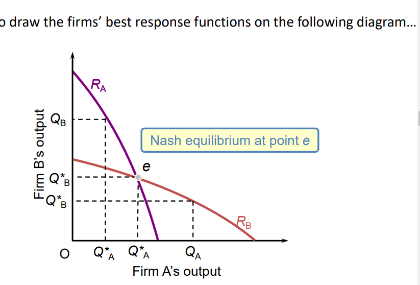
Cournot Nash equilibrium

when no firm wants to change its output level holding both output levels constant

equilibrium is at the intersection of both firms best response functions on a diagram

(made up of tracing the different output levels using the marginal output rule MC=MR and the differing demand curves based on what the the other firm produces)

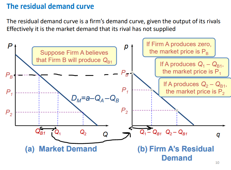
residual demand curve

a firms demand curve given the output of its rivals

the more firms B produces the closer firm A’s residual demand curve is to the origin

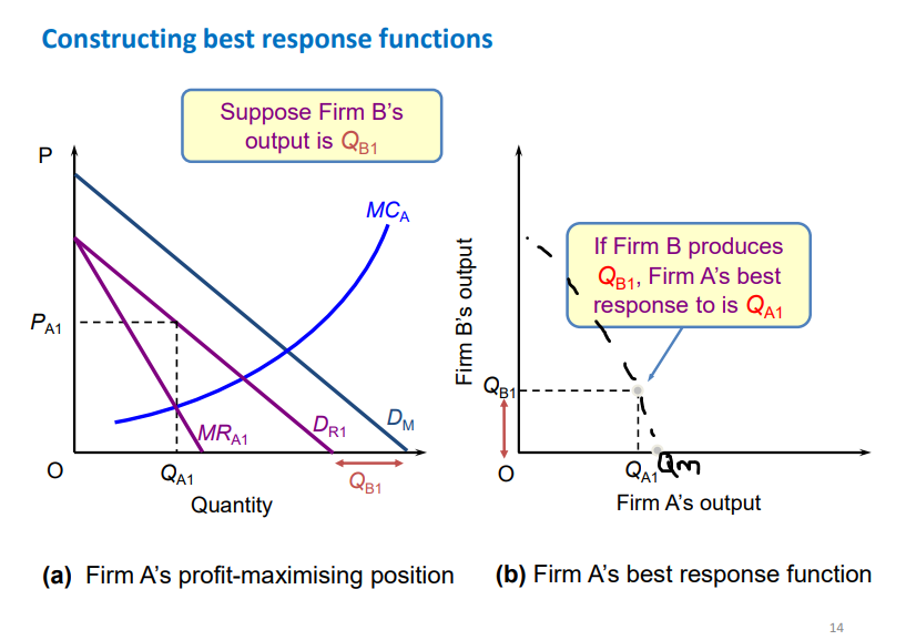
constructing Cournot best response functions

made up of tracing the different output levels using the marginal output rule MC=MR and the differing demand curves (original demand versus different residual demand curves) based on what the other firm produces

if firm B doesnt produce anything firm A produces at monopoly output Qm with normal demand curve, if firm B produces Qb1 output is at residual demand curve so firm A produces Qa1 which is lower than Qm.

profit increases as output tends towards the monopoly level

comparing Cournots oligopoly to monopoly and perfect competition

• the duopolists ( 2 firms) together produce more than 1 monopolists would produce

• the market price is lower than for a monopoly but higher than perfect competition = profit making

Bertrand’s oligopoly model assumptions

• there are only 2 firms in the market (duopolists), they choose level of price (compete in prices) and make their pricing decisions simultaneously

• further entry into the market is completely blocked

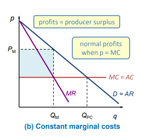
• firms have the same constant marginal costs and no fixed costs (which means Total costs = variable costs, and average costs = marginal costs)

• firms produce identical products (so buyers purchase from cheapest seller)

• market demand: Q = a - P (subtract firm A’s price when its below firm B’s and subtract firms B’s price when PA is above PB)

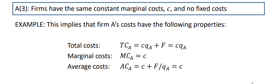
constant marginal costs

bertrand nash equilibrium

when no firm wants to change its price

equilibrium consists of price pA and pB such that given fir bm B charges pB, firm a profit max price is pA, and given firm A charges pA, firm B’s rpfoit max is pB

the intersection of firm A and B best response functions

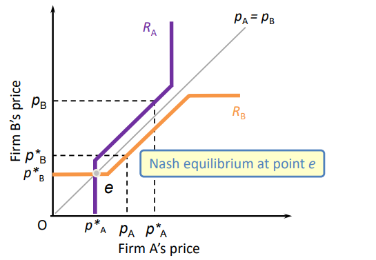
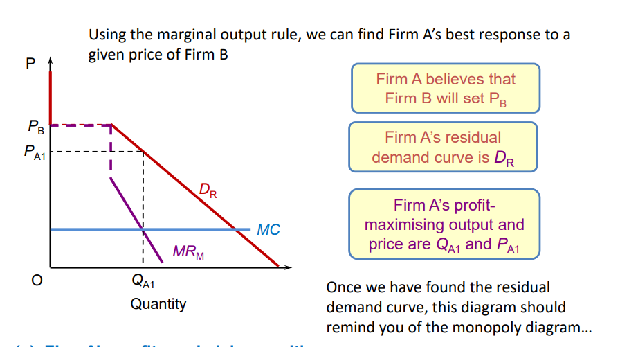
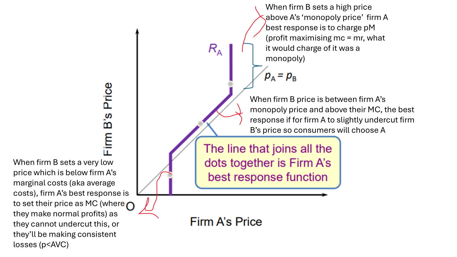
Betrand firm specific demand curve and pmax position

if firm believes firm B will set a certain price, under the assumption that their products are identical, consumers will not buy from firm A if their price exceeds that of firm B, so demand curve cuts off at firm B price and is 0 (as firm A sells nothing)

bertrand best response function points explained

Bertrands model compared to monopoly and perfect competition

• set a lower price than the monopoly level

• market produces more output from the duopoly than under a monopoly

• set same price as in perfect competition (no deadweight loss)

• bertrands total welfare is consumer surplus

what is the bertrands paradox?

• the model claims that by adding only one firm we go from the extreme of monopoly to the other extreme of perfect competition

• this is not seen in reality

ways to break the Bertrand paradox

1) if we account for PRODUCT DIFFERENTIATION a seller won’t lose all their customers when their rival has a higher price

2) consider CAPACITY CONSTRAINTS as even if all buyers go to the firm with the cheaper price, the firm may not have the ability to supply the whole market

3) acknowledge there is INCOMPLETE INFORMATION about prices and costs so even if a firm has a lower price, consumers may not know so wont all flock to the cheaper firm

4) firms may not compete as intensely as the Bertrand model predicts if they INTERACT REPEATEDLY as they may recognise their ability to charge higher prices if they compete less

what is the prisoners dilemma? solution?

the prisoners dilemma is where the dominant strategy for both players is to act with self interest, but this leads to a nash equilibrium with a less than optimal payoff

to solve this dilemma, players can cooperate to both get a better payofff

however when firms agree to cooperate there are short term incentives to deviate from the agreement to gain an even higher payoff

oligopolies methods of collusion in cournot and bertrand models

• for Cournot (quantity setting model) if the firms cooperate they can both produce half of the markets monopoly profit max quantity

• for Bertrand (price setting model), both firms can produce at monopoly price

• for both there is a short term incentive to produce more than their share of the monopoly quantity to increase profits, or to just undercut the monopoly price by a small amount to encourage more consumers

conditions necessary for oligopolists to collude

1- sellers must interact repeatedly → this means the incentive to deviate from the cooperation agreement will be counteracted by a long-term punishment such as price wars (with price wars the profits from deviating in the long run decrease)

2- sellers must be aware of each others strategies → so will be aware of deviation and bale to punish it, firms may form cartels to monitor firms and make sure they’re each conforming to the agreement

grim trigger strategy

if both firms have decided to cooperate, as soon as one player deviates the firms revert to playing the one-shot nash equilibrium deviate, deviate forever (As trust is lost between the firms so will no longer agree to cooperate)

infinitely repeated prisoners dilemma nash equilbrium

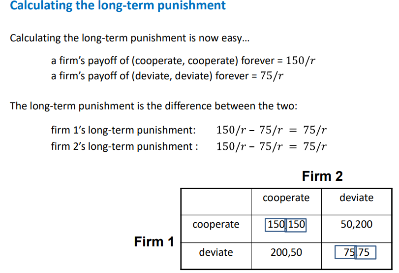
cooperate, cooperate is the forever nash equilibrium if the short term benefit from deviating is less than the long term punishment

short term benefit: difference in payoff between cooperate, cooperate and deviate, cooperate (what they gain by breaking the agreement)

long-term punishment: the difference between a firms payoff from cooperate, cooperate / interest rate (dividing by interest rate helps put future payoffs as present values to represent long-term) and a firms payoff from deviate, deviate / interest rate → if interest rates are HIGHER the firm is more likely to deviate as it’s more attractive to gain higher payoffs now

finitely repeated prisoners dilemma

can use backwards induction to find a nash equilibrium in each subgame

Supply of labour by an individual worker

supply is upwards sloping (usually) or backwards bending (rarely) depending on which effect dominates:

• substitution effect: at higher wages a person will work more as leisure has a greater opportunity cost (losing out on more income with same leisure time)

• income effect: higher wages imply worker can afford more leisure time (if dominates = backward bending)

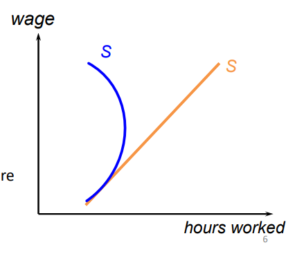
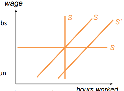
supply of labour to an employer

an employers labour supply depends on whether employer is a wage taker (curve will be perfectly elastic) or a wage maker (upwards sloping)

shifts in supply curves due to:

• changes in number of qualified people

• non wage benefits attracting employees

changes in slope (responsiveness of supply to wage changes) depends on:

• the difficulty of changing jobs

• short-run vs long-run

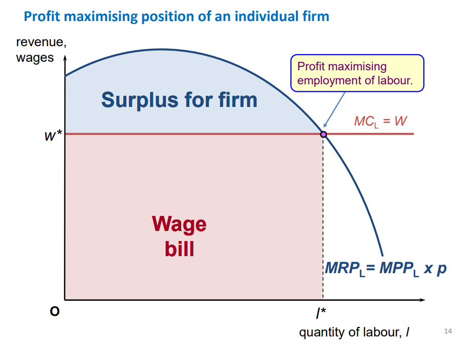
marginal input rule

a firm should employ the number of units of labour where MRPL, marginal revenue product of labour = MCL, marginal cost of labour

MRPL is the change in revenue from employing one more unit of labour

MCL is the change in total costs from employing one more labour unit

Assumptions of perfectly competitive labour markets

• firms operate in a perfectly competitive OUTPUT market (so they’re price takers, can sell as much output without affecting price, and MRPL = p x MPPL)

• firms are wage takers in the labour markets (employ as much as want and wont change wage, MCL = wage rate)

• both buyers and sellers (firms and workers) have complete information, workers know available jobs, employers know how productive the available labour is etc.

• workers are wage takers (no matter how much labour they supply wont affect wage rate)

• entry for workers is free, no restrictions on labour movement (assumed long run as takes time for workers to become educate etc.)

market structure of perfectly competitive labour market

• many small number of workers

• low barriers to entry

• undifferentiated workers, firms consider all workers to be identical so employ the cheapest (could differ due to productivity, ability, experience differences)

• many small number of firms

profit maximising employment of labour for wage taker firm

where MRPL and MCL intersect, with MCL/ wage rate being constant as firm is a wage taker

when is the labour market in equilibrium

when firms (buyers of labour) optimal employment level is equal to workers (sellers of labour) optimal supply levels given the market wage

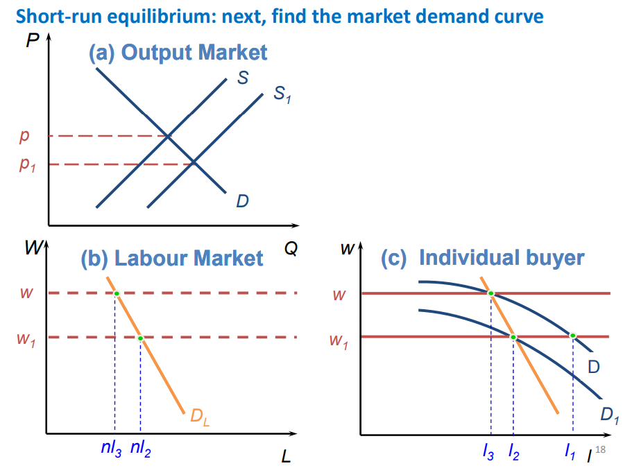
short-run equilibrium in labour market, diagram and what determines it

the equilibrium price of the goods is determined by supply and demand in the output market

this price determines the MRPL for an individual buyers of labour which determines demand (as demand and MRPL are equal)

The labour demanded by an individual buyer at each wage rate is determined by the subsequent change in price (as if wage rate decreases, supply of output increases which causes price to fall) which shifts the Demand/MRPL curve down)

the number of firms in the market (n) multiplied by the labour each firm demands at each wage rate (L, L2, L3 ETC.) makes up the labour demand curve in the labour market

then you add the labour supply curve and the intersection determines the short-run equilibrium

monopsony

when there is one large buyer of a particular good or service

NOTE: monopsony firm in labour market DOES NOT MEAN it must be a monopoly in output market

wage making employees

when employees have the power to influence the wage rate they receive due to:

having a unique talent

creating a union and threatening action (E.g. strikes) if their demands are not met

examples of imperfect labour markets

• when the firm is a monopsony and therefore a wage maker in the labour market

• firm as a discriminating monopsony (pay workers different wages depending on the lowest wage each worker is willing to accept

• monopoly union labour market → workers form together to form a union where they are wage makers (have influence on wages)

• bilateral monopoly → where BOTH firms AND workers are wage makers

assumptions of monopsony labour market + market structure

• firm is a price taker in OUTPUT MARKET (perfect competition)

• firm and workers have complete information

• workers are wage takers

• free entry for workers

• firm is a WAGE MAKER in labour market

Market structure:

many small sellers (workers), and one large buyer (firm)

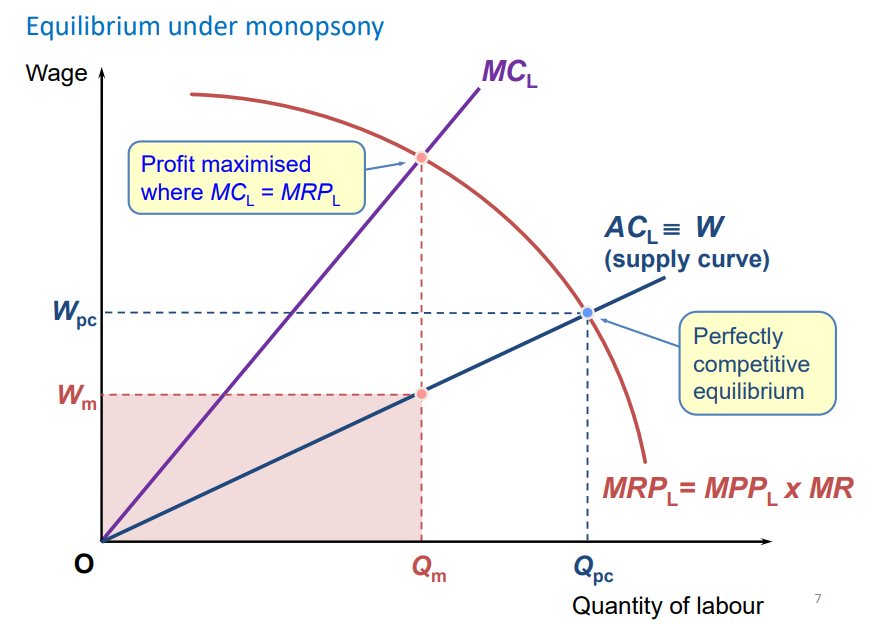
equilibrium/profit maximising quantity and wage in monopsony labour market (+ difference to perfect comp)

supply curve is upwards sloping as attract more workers at higher wage.

TC = wL so AC = wL/L = w (wage rate)

supply = AC = wage rate

MC is greater than AC

marginal input rule: profit maximised at MRPL = MCL, trace down to supply curve to find equilibrium wage rate

lower wage rate and lower quantity to perfect comp → deadweight loss

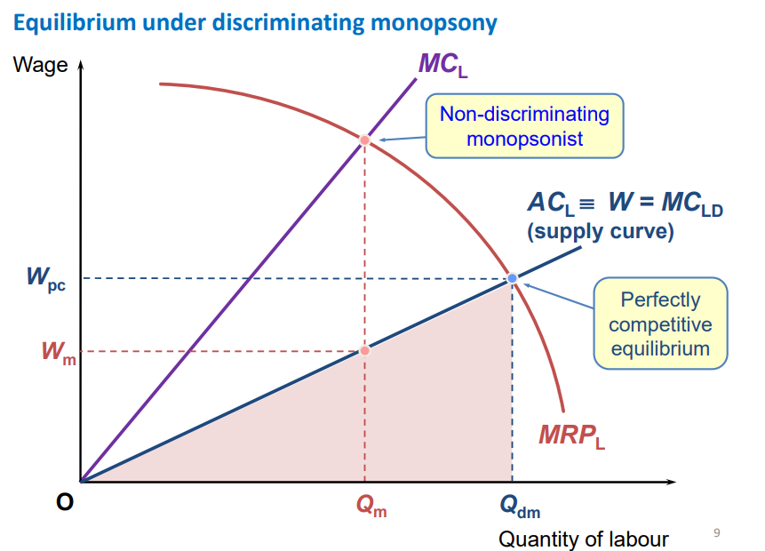
discriminating monopsony labour market

this leads to Marginal Cost being equal to Average cost

(because when a new worker enters, TC increases by the wage that new worker is willing to accept, rather than ALL wages changing to match the different rate)

produce where MC = MRP → so produce SAME QUANTITY as perfect competition but at varying wages

no deadweight loss

monopoly union labour market assumptions and market structure

• firm is a price taker in OUTPUT market

• firm and workers have complete information

• firms are WAGE TAKERS

• workers are WAGE MAKERS → assume union sets a minimum wage and are commonly interested in maximising wages for members or maximising employment

market structure:

one large seller = union (coordinated action so workers seen as one big group)

many small buyers (firms)

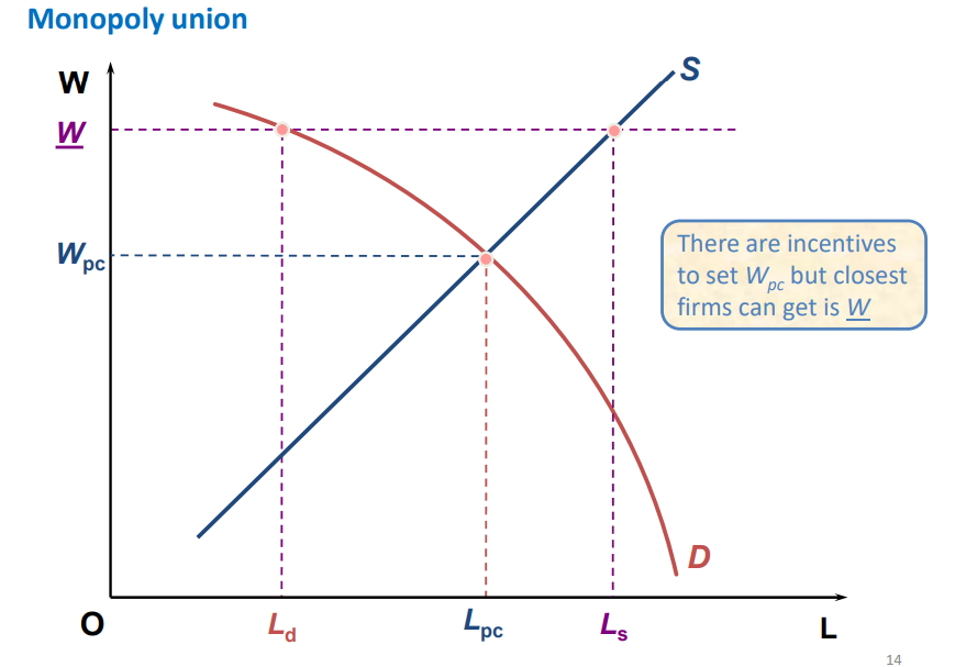
monopoly union diagram

sets minimum wage above equilibrium wage

causes excess supply = unemployment (difference between Ls and Ld)

because rise in wage increases firm costs which shifts supply in output market → demand less labour in labour market (from Lpc to Ld)

Bilateral monopoly assumptions + market structure

• firm is a wage maker

• workers are wage makers

• firm and workers have complete info

• firm is a price taker in output market

market structure:

one large seller (Worker union) and one large buyer (firm)

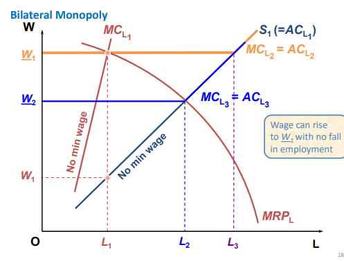
bilateral monopoly diagram

wage can rise to W1 with no fall in employment as intersects where MRPL = MC (which is same quantity firm employs as a monopsony)

BEST to set minimum wage at W2 (where perfect competitive wage is) as this increases wage (From W1) and INCREASES employment

efficiency vs equity

efficiency and equity determine whether something is SOCIALLY DESIRABLE

efficiency is about how well resources are allocated to produce the best amount and it’s objective

equity is about fairness in distribution and is subjective

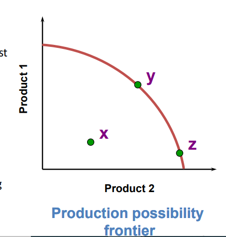
Types of efficiency + PPC

• productive efficiency: how resources are allocated within a firm and among different firms so that each firm is producing at the lowest cost possible → on PPC any point along the curve (y, z etc.) is productively efficient as this the max that can be produced when efficient

• allocative efficiency: when gains are maximised so no more gain can be made by further reallocating resources → this is dependent on what benefits society e.g. if product 2 is better for society z would have allocative efficiency while y only has productive efficiency

Pareto optimality vs Pareto improvements

Pareto optimal: when it is not possible to make one better off without making another worse off (allocation of resources are efficient

Pareto improvement: allocation of resources is not fully efficient as it is possible to make one better off without making another worse off

NOTE: both occur in the absence of the other e.g.no Pareto improvements to be made when there is Pareto optimal allocation and vice versa

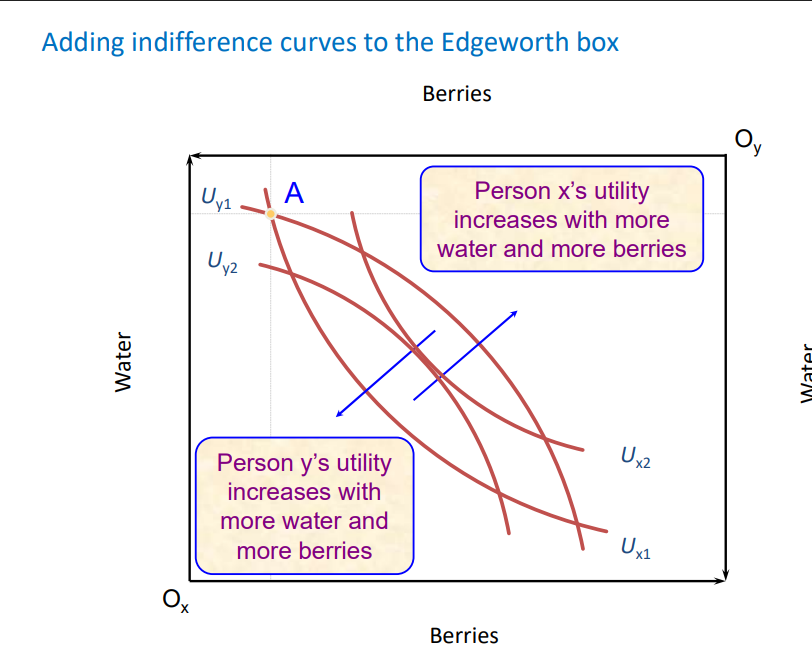
Edgeworth box

shows every possible outcome from trade between x and y to show how resources can be allocated

draw in the indifference curves for each remembering that further away from origin the higher the utility

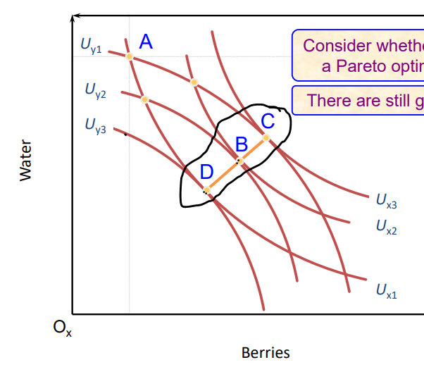
Pareto optimal resource allocation in Edgeworth box

Along the Core (D,B,B C) there is Pareto optimal allocations

as to get from any point across the core you need to make one worse off

e.g. for point D, to increase Ux you need to decrease Uy so from D to B Ux1 increases to Ux2 while Uy3 falls to Uy2

private and social efficiency

private efficiency: when marginal private benefit = marginal private cost → seen in competitive markets

social efficiency: when marginal social benefit = marginal social cost → when trade has no effect on third parties (externalities), same as Pareto optimality

what are externalities

external benefits and costs

they imply that social benefits and costs diverge from private benefits and costs SO market leads to a point that is privately efficient but not socially efficient = market failure

characteristics of externalities

→ can be positive or negative: positive means there is an external benefit and these goods are underproduced in the market; negative means there is an external cost and these goods are overproduced in the market

→ can be production e.g. honey producers promote bees good for pollinating flowers or consumption e.g. vaccination externalities

→ to respond to negative externalities don’t just ban all goods but find best trade off between benefits and costs (so produce at socially optimal quantity → more desirable)

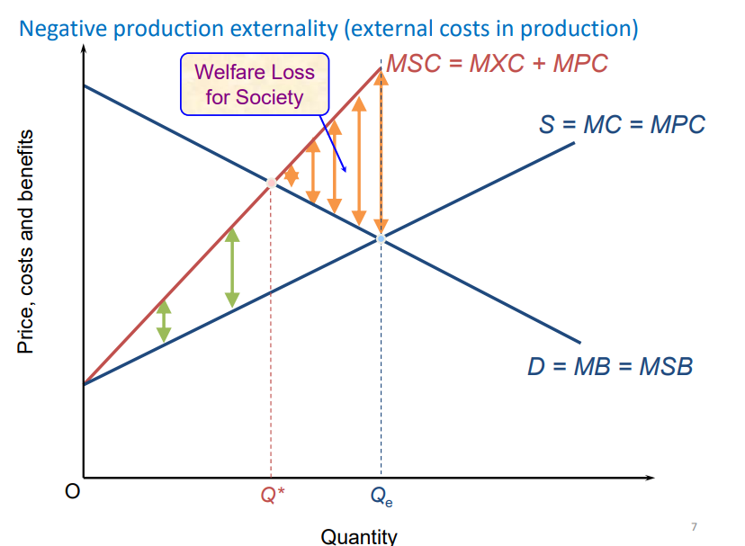
negative production externality diagram

MPC exceeds MSC, the tilt instead of parallel indicates that the more the good is produced the bigger the externality

welfare loss triangle points towards Q* (socially desirable Q)

MSC = Marginal eXternal Costs + MPC

Qe is privately efficient and is more that socially efficient Q* as good is overproduced

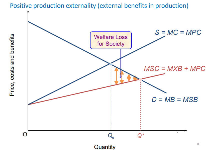
positive production externality

production of good has external benefits so MSC = MPC + Marginal eXternal Benefits

MSC exceeds MPC

Qe (actual quantity produced) is lower than socially efficient quantity = underproduced

negative consumption externality (FROM TEXTBOOK)

positive consumption externality (FROM TEXTBOOK)

Ways to correct externalities

1. Market based policies

• Pigovian taxes to discourage production/consumption e.g. sugar tax

• subsidies to encourage production

this can INTERNALISE the externality by attempting to align private incentives with social efficiency → so want firms to consider their effect on society and increase/decrease production accordingly

2. Regulation e.g. quotas

why market based policies over regulation? (pollution example)

• the tax would reduce pollution more efficiently

• the tax can be better for the environment as it gives an incentive to reduce pollution as much as possible (regulation means likely to just reduce up til point)

• tax raises revenue for the government (they can put this towards reducing pollution further)

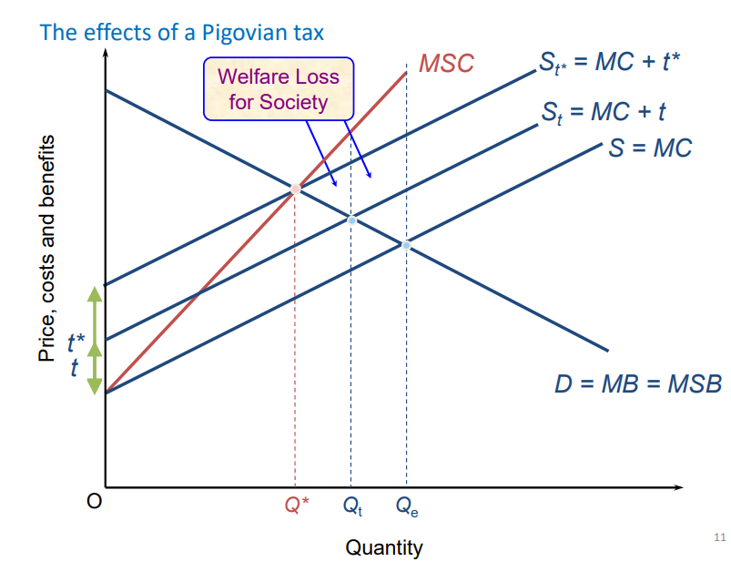
Effects of a Pigovian tax diagram

with tax production decreases so PC falls (shifts left) to MC + t, welfare loss gets smaller

aim is to charge optimal tax rate: t* so that new supply curve meets at same point as MSC and MSB socially efficient point

Rival products

• some rival goods can only be consumed by one person e.g. petrol

• some rival goods can be consumed by more than one person but NOT at the same time e.g. laptop, use it and then sell 2nd hand

• some rival goods can be consumed by more than one person at the same time but the number is limited and others may still be restricted from consuming the good e.g. a football stadium has limited seats,

If these don’t apply the product is non-rival e.g. fireworks can be enjoyed by anyone around

Excludable products

excludable products are products which non-payers can be excluded from consuming (still excludable whether or not person is actually excluded e.g. doctors appointments can be excluded but may not be)

non-excludable is when you cant be prevented from consuming a product if you refused to pay

→ difficult to distinguish between excludable and non-excludable, and changes in technology can transform a good from non-excludable to excludable (e.g. TV channels have developed to have options to pay for certain ones)

4 types of goods

free rider problem + solution

a free rider is a person who receives the benefit of a good without paying for it e.g. fireworks, one person pays and the free-riders also enjoy the show → the case for non-excludable goods

due to the free rider problem public goods are under produced by firms or not produced at all as despite value to society = market failure

solution: government pays for and provides the public goods and handled costs through tax revenue

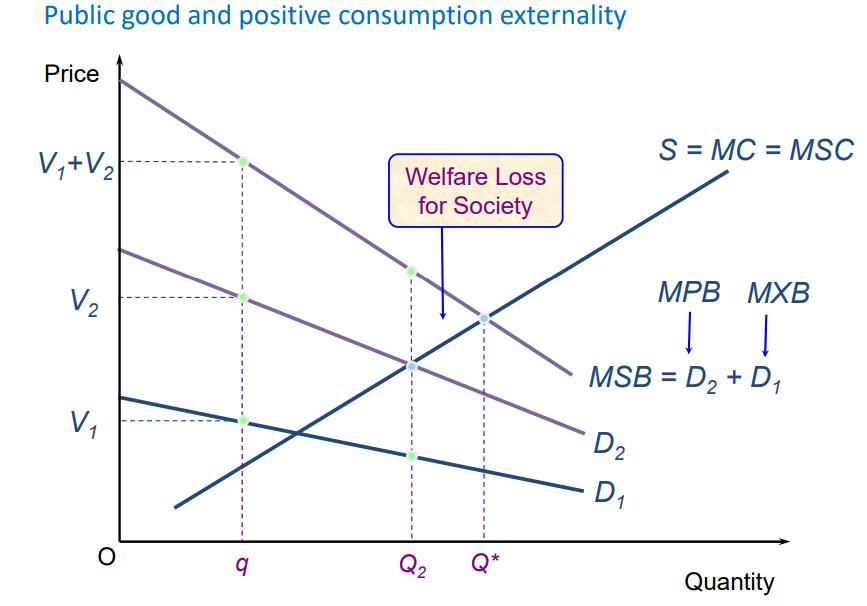
public goods market failure diagram

free ridder problem can be viewed as a positive consumption externality

D1 represents the free riders who experience the external benefits (MXB) without paying for the good

production occurs at MSC = D2 instead of MSC = MSB (= D2+D1) as D1 doesnt pay for the good when they can be a free rider

this leads to underproduction and a welfare loss