Chapter 11 - Further Matrices

Following up from Ch 10 - in a nutshell (of course, literally)

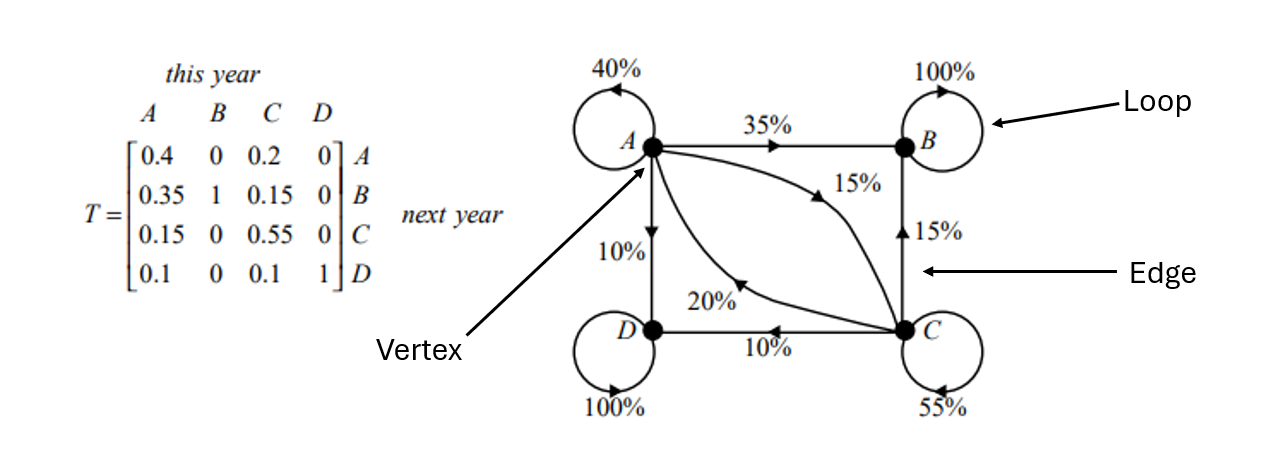
Transition Matrix

• Represents how states change from one to another over time

• Square matrix with proportions (decimals), showing percentage chances

• Used in systems like weather prediction or state transitions

• Visualized as a directed graph: vertices = states, edges = transition probabilities

• Columns = Starting states (where you begin)

• Rows = Ending states (where you end up)

• Each column sums to 1 (100% of probability spreads out)

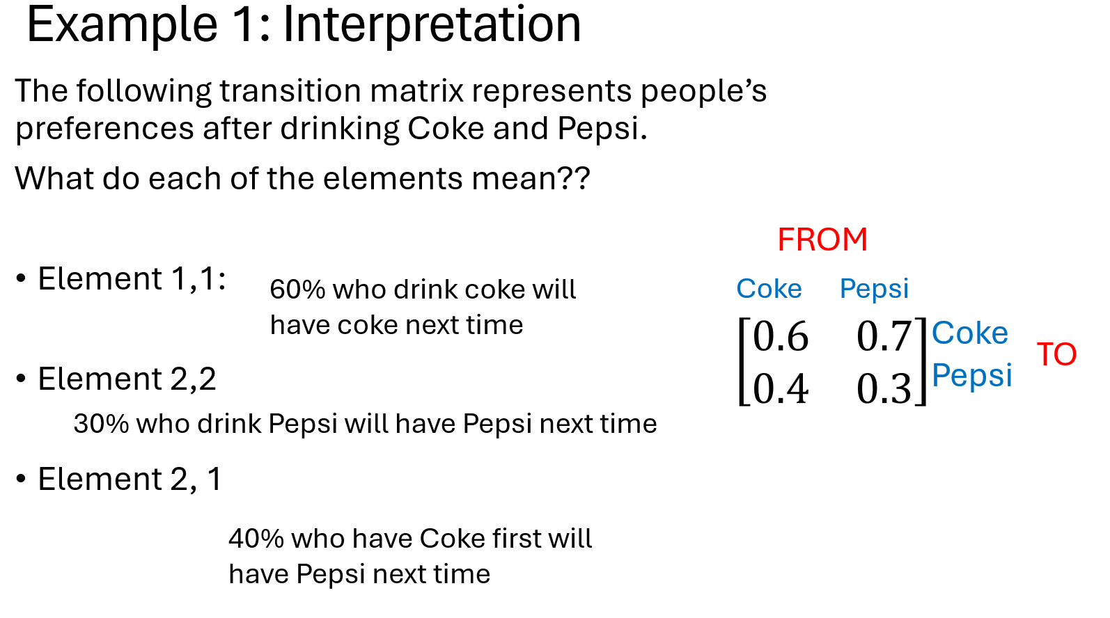
Interpretation of Transition Matrix: Example

State Matrix

• Transition matrix = proportions moving between states

• State matrix = counts/items in each state at a time (column matrix)

• Initial state matrix (S₀) = starting counts

• Example:
  S₀ = [50 40] for Bendigo (B) and Colac (C)

• Labels match those in the transition matrix for clarity

Be Careful with State Matrix!

• Initial state matrix varies by question — always check what time it represents (start, after 1 week, etc.)

• Identify the correct starting point before applying transitions

• Time changes = multiply by transition matrix the right number of times (e.g., S₁ = Transition × S₀, S₂ = Transition² × S₀)

• Don’t assume initial = time zero unless stated!

Transitions and State Matrices

• To find next state: Sₙ₊₁ = T × Sₙ

• Start with S₀ (initial state)

• Multiply by T (transition matrix) to get state after 1 step (S₁)

• Repeat for continuous steps:

  • S₂ = T × S₁

  • S₃ = T × S₂, and so on...

• Pre-multiply every time (transition matrix goes before state matrix)

• Each multiplication redistributes objects according to transition probabilities

Rule for Finding the State Matrix

n = number of time periods (days, months, years, etc.)

To find state after n steps:

Sₙ = Tⁿ × S₀

• Raise the transition matrix T to the power n (use CAS or by repeated multiplication)

• Multiply by the initial state matrix S₀

Result: state distribution after n transitions

Steady State Matrix

• The point where objects keep moving but overall numbers at each point don’t change

• Happens when leaving = arriving at every point

• Requires:

  • Regular transition matrix (powers have no zero elements)

  • Columns sum to 1

• Found by letting n → ∞ in 𝑆ₙ = 𝑇ⁿ𝑆₀

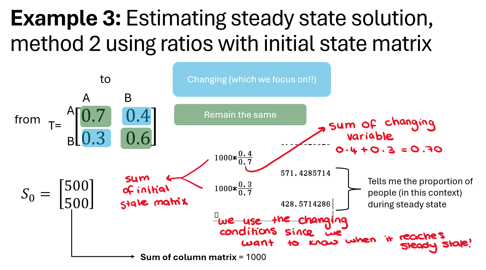
Finding Steady State Using Ratios (2×2 Matrices Only)

• Used when steady state is known but transition matrix is unknown

• Set the steady state proportions as variables (e.g., x and y)

• Use the fact that in steady state, inflow = outflow for each state

• Write equations based on transition probabilities as ratios between x and y

• Solve for the ratio x : y to find steady state distribution

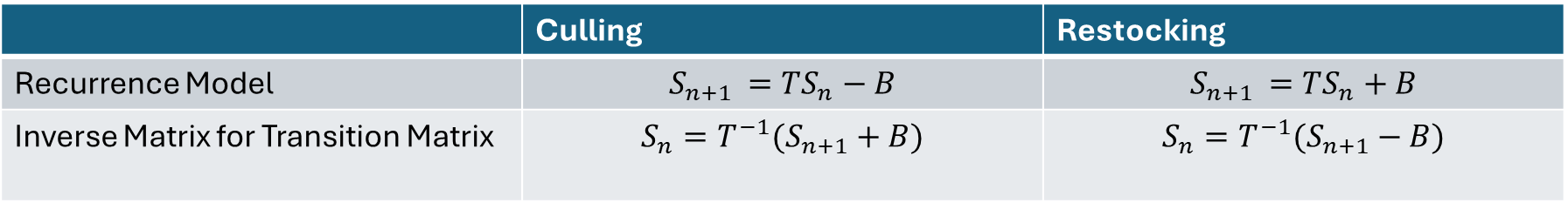
Changing Values in Recurrence Relation

• Normal rule:
  S₀ = initial state
  Sₙ₊₁ = T × Sₙ (population constant)

• When population changes by fixed amount:
  Sₙ₊₁ = T × Sₙ ± B
  B = column matrix with fixed additions/subtractions

• Culling:
  Taking away items → B is negative

• Restocking:
  Adding items → B is positive

• Rearranged equation:
  Sn = T⁻¹ (Sn+1 − B) → Make sure that this is in brackets and DO NOT do it step-by-step basis

General: Culling / Restocking

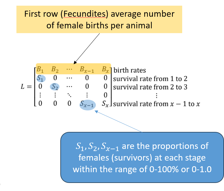
Leslie Matrices (L)

• Special transition matrix modelling population changes over time (ignores migration).

• Focuses on females only (birth givers).

• Population split into equal-length age groups covering lifespan.

Key factors for each age group iii:

• Birth rate b_i: average number of female offspring per mother in age group iii per time period.

• Survival rate s_i: proportion of females in age group iii who survive to age group i+1 (Note 0≤s_i≤1).

Leslie matrix tracks birth + survival across age groups.

Leslie Matrix Quick Guide:

• First row: Birth rates (fecundities) — average female offspring per age group, can be >1 or 0 if no births.

• Subsequent rows: Survival rates — proportion moving from one age group to the next (0 to 1).

• Last row: Survival of oldest group, either 0 or feeding back into itself if they survive another period.

Key: Births at top, survival flows down.

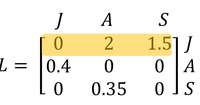
Interpreting Leslie Matrices: Dung Beetle Example

Age groups: Juvenile (J), Adult (A), Senior (S)

First row (Fecundity): Average offspring per age group — controls next Juvenile population size

• l₁,₁: Juveniles = 0 (too young to reproduce)

• l₁,₂: Adults = 2 juveniles each

• l₁,₃: Seniors = 1.5 juveniles each

Into Adults (Row 2): Transitions into Adults

• l₂,₁: 40% of Juveniles become Adults

• l₂,₂: 0% Adults remain Adults

• l₂,₃: 0% Seniors become Adults (no backward aging)

Into Seniors (Row 3): Transitions into Seniors

• l₃,₁: 0% Juveniles become Seniors (no skipping stages)

• l₃,₂: 35% Adults become Seniors

• l₃,₃: 0% Seniors remain Seniors (no staying unless specified)

Key points:

• High fecundity → fast growth, good replacement, less extinction risk

• Low fecundity → slow recovery, risk of decline or extinction

Fecundity row is the heartbeat of survival — it shapes the future population flow.

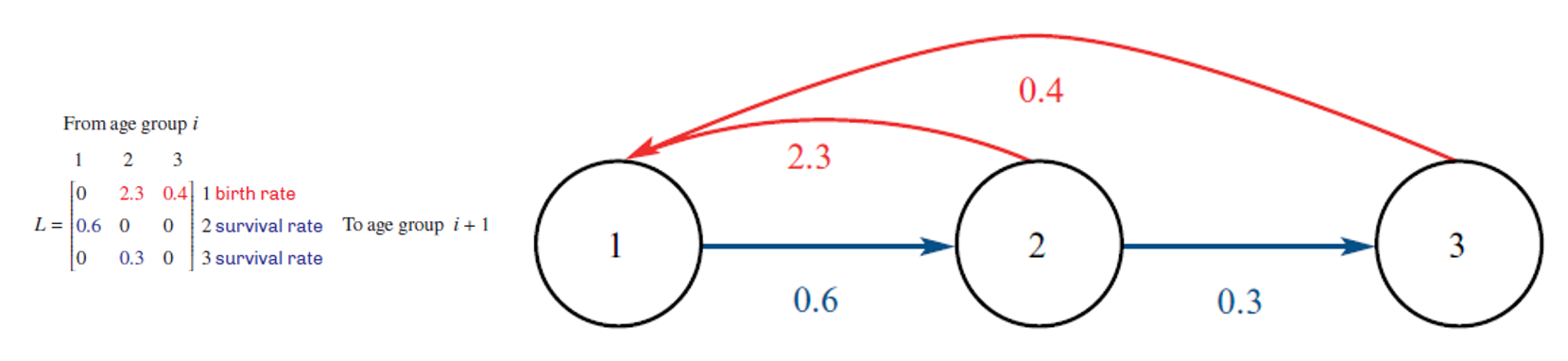
Leslie Matrix Life Cycle Diagram

• Horizontal arrows: Show the proportion of each age group that progresses to the next stage.

• Back arrows to first age group: Represent the number of offspring produced by each age group.

Recurrence Relation / Rule for leslie state matrix

Recurrence Relation (step-by-step movement):
S₀ = initial value, Sₙ₊₁ = L × Sₙ

Rule for finding the state matrix:
Sₙ = Lⁿ × S₀

Same steps as with transition matrices — just swap in the Leslie matrix (L).

Population State Matrix

A column matrix showing the number of individuals in each age group at a given time.

• The initial state matrix is S₀.

• Example: If there are 400 females in each age group at the start:
   S₀ = [400

  400

  400]

Each step forward uses: Sₙ₊₁ = L × Sₙ.

Long-Term Trends with Leslie Matrices (m × m)

• Increasing population → if Sₘ > S₀

• Decreasing population → if Sₘ < S₀

• Cycling/oscillating population → if Sₘ = S₀, repeats every m steps
   ➡ Happens when: Lᵐ = I (identity matrix)

Check Sₘ after m time periods to detect trend.

Growth Rates (Limiting Behaviour) – Leslie Matrices

• Populations don’t reach steady state, but reach proportional equilibrium

• Proportions in each age group stabilise, even if total numbers change

• This is called the long-term growth rate, denoted by g

Rule:
If for all elements:
Sₙ₊₁ / Sₙ = same value = g

Then:

• g > 1 → Population increases

• g < 1 → Population decreases

• g = 1 → Population is stable

Formula:
L × Sₙ = g × Sₙ₋₁

g = growth rate of the population each time period
To find % growth: (g − 1) × 100%
g must be a real number