midterm 2

Classical test theory

X = T + E

X; obersved score

T: true score

E: error

KEY observed score is the sum of the true score and some error

parallel forms (CTT)

two forms measure the same construct with equal true scores for each person and equal error variance.

NOTE: true score is constant across forms Tij = Ti and the error term Eij is random

For Classical test theory what do we collect?

an observation for participant i, we get a different value for Xij because of the error term Eij

Eij ⊥ Tij

Error term Eij is random. it is independent of (__) the true score Tij

Eij ∼ Normal(0, σ2E )

error term Eij is normally distributed with mean 0 and variance σ2E

implies that error has an EXPECTED VALUE of 0

E[Eij ] = 0

What is observed Score Distribution (CTT)

implies that the observed scores are also random variables that follow a normal distribution

• each person hsa own FIXED TRUE SCORE Ti

• ERROR term Eij is randomly sampled from a Normal(σ2E)

• composed by constant true score Tij = Ti and random error term Eij

• IS REPEATED measurments is centerd around the true score Ti with some random error Eij

  
  

Xij ~ Normal(Ti, σ2E)

Expected Values (CTT)

E[X ] of any variable X is the expected long run average if we could repeat the measurment infinitely many times (the mean of the observed scores would be the true score)

Normal random variable is it mean E[X ] = μ

In CTT: Xij - Tij + Eij

EX of true score: E[Tij] = Ti (constant for person i)

Ex value of the error: E[Eij]] = 0

Ex: value of the observed score: E[Xij] = Ti — the mean of the observed scores would be the true score

Variance decomposition (CTT)

Var(Xij) = Var(Tij) + Var(Eij)

Var(Tij) = 0 → people true score is constant Tij = Ti

Var(Eij) = σ2E → random error fluctuations

Var(Xij) → variability inherited from Tij and Eij

SAME AS: Var(Xij) = σ2E

Xij ~ Normal(Ti,σ2E)

Full decomposition (CTT)

single participant i taking parallel forms of a test j: recall Xij = Ti + Eij

Expected values: E[Xij] = E[Tij] + E[Eij] = Ti + 0 = Ti

Variance decomposition: Var(Xij) = Var(Tij) + Var(Eij) = 0 + σ2E = σ2E

Measurement Error

refers to the difference between a measured value and the true, or actual, value of what is being measured

IS INEVITABLE/imperfect

EXS: fluctuates weighins, blood pressure cuff (different readings), reaction time task (attention/fatigue)

how does measrument error effect repeated scores for one individual?

the is variability across participants’ Ti, so we treat Ti as a random variable Ti ~ Normal(μT , σ2T)

intro a new source of variance: σ2T (true score variance across people)

within one participant (fix = i Juan)

Model (parallel forms): XJuanj = TJuan + EJuanj

TRUE SCORE (constant for i) = E [XJuan,j ] = TJuan, Var(TJuan) = 0

ERROR: E[Ejuanj] = 0, Var(Ejuanj) = σ2E

Variance (within i): Var(XJuanj) = σ2E

Across partiipants (i = 1,….,n)

true scores vary between people: Ti ~ Normal(μT , σ2T)

observation model: Xij = Ti + Eij

Expectaions: E[X] = μT

Variance(across people & forms): Var(X) = σ2T (← true difference) + σ2E (← measurement error)

multiple participants

each people “i” has their own true score Ti (varies across people, constant within person)

Each observation adds random error Eij (varies across forms/replications j)

oberved score: Xij = Ti + Eij

true scores vary sysmtematically

Ti ~ Normal(μT , σ2T)

each observation adds unsystematic error: Xij = Ti + Eij , Eij ~ NOrmal(0,σ2E)

what does Var(X) reflects for multiple participants

both systematic differences between people and random fluctuations within people

Random error / Random variation (σ2E)

unpredicatble (sign/magnitude from trail to trail)

AVERAGES TO 0 : E[Eij} = 0

Inflates Var(E) → lowers reliabilty

Ex: momentary distraction, room noise, hand timing jitter , recation time task, blood pressure reading, essay grading, quntionnaire

Systematic error / Systematic variation (σ2T or bias)

CONSISTENT SHIT (drift/offset) or stable between person differences

DOES NOT AVERAGE TO 0 (correltae with other variables)

if RELATED TO MEASUREMENT bias if threatens VALIDITY more then realiability

Ex: Culturally loaded items, fixed order effects, miscalibrated thermometer, survey wording, test instructions, stopwatch

CREATE BIAS AND THREATEN VALIDITY

Reducing Random Error

increasing test length with quality items E[Xij] = E[Ti]

Averaging/aggregation to cancel noise

standardize instructions, timing, environment

USE clear, unambiguous items; pilot and reivse

Train rates, use rubrics and double scoring to stabilize judgements

Mitigating Systematic Error (Bias)

Calibrate device; check drift regularly

Randomize item/order (counterbalance)

Neutral wording: avoid leading or culturally loaded content

Analyze DIF/fairness across groups; revise baised items

Thought experiment

measure you own anxiety level 5 times within a day

if true anxiety is table than within person reflect random error

if measruemtn steadily increase a caffeine wears off then systematic component

averaging the 5 measruments reduces random error (law of large numbers) but does not fix systematic bias

Signal vs. Noise

obsered variance has two components:

Var(X) = σ2T + σ2E

σ2T : true variance (systematic)

σ2E: error variance (random)

Reliability as a Ratio Variances

reliability tells us the proportion of observed variance that reflects true differences between people, rather than random error

values range from 0 to 1:

0 - all variance is NOISE (no measurment)

1 - all variance reflects TRUE SCORES (perfect measrument)

higher reliability indicates more consistent, dependable measurements

CTT MAIN ASSUMPTIONS

E{E} = 0 (across many replications, error averages out)

E⊥ T (error is uncorrelated with true score)

parallel replication of the same test (or parallel forms) target the same T

Parallel forms (test forms in CTT)

two forms measure the same construct with equal true scores for each person and equal error variances

EX: two alternate versions of an exam with equally difficult items and identical score distributions

Tau equivalent forms (test forms in CTT)

true scores may differ by a constant shift, but all forms are on the same scale. Error variance may differ

Ex: two math test with same degree but one test is burrly than the other

Congeneric forms (test forms in CTT)

all forms measure the same construct, but may differ in both scaling (factor loadings) and error variances

Ex: depression questionnarie like “i feel hopeliess” is strong indciator while “i have trouble sleeping is weak and more influenced by other factors

(Reliability coefficients rely on different assumptions about equivalnce between items or forms)

What is a psychological scale?

measrument instrument designed to collect observable indicators for psychological latent constructs

Ex: personality traits, attributes, beliefs/attiudes

collected through items, meaure different aspects of the construct of interest

— repsonses given by respondents across these items are COMBINED to produce one general measure of the construct of interest (scale score)

Scale scores

different repsonses given by a participant across all items are combined to obtain a measure of the construct of interes

Ex: all items combined into total score, report separate subscale scores, reported in standardized untis, or in cut-offs

Examples of psychological scale

Beck depression inventory - 21 item scale

Big five inventory - 50 item scale

Rosenberg Self Esteem scale - 10 item scale

Perceived Stress scale - 10 item scale

Hamilton anxiety rating scale - 14 item scale

psychological scales in action

clinincal settings (mental health), research (construct of interest), education(leanring), industrial(employee satisfaction), government (public opinoin), non-profit (effectivness)

Scale development: the Big picture

1. define the construct and its content domain

2. generate items

3. expert review

4. cognitive interviewing

5. scoring plan

Scale validation

5. pilot study

6. item analysis

7. dimensionality

8. reliability

9. validity evidence

10. scoring definition

11. finalize & document

Step 1: definining the construct and domain

Step 1.1) name & purpose:

• clearly state the construct we want to study

• if broad than difficult to provide full account of its different compoents

• if too constrained then difficult to desgn items that measure different aspects

  identify the intended use of the scale (ex clinical,product placement, exploratory)

Step 1.2) working defintion

1. general description of the CORE phenomeon

2. unit of analysis (attidues, behaviors, belifs) used to study it

3. Reference period (past 2 weeks) and stbility expectations

Step 1.3) identify the content domain (factes):

Enumerate non overlapping facts

Write a bief not for each facet

Ex: test anxiety — negatieve thoughts, physiological arousal, cognitive interferene

use these facts to write items that measure different aspects of the construct domain

Step 1.4) define the construct’s boundaries (out of scope)

CLARITY what is NOT included, even if it look similar

Helps avoid item drift, construct contamination, and overlap with other measures

boundaries ensure the scale measures the intended latent trait rather than related but distinct constructs.

Ex: test anxiety (boundaries) — generalized anxietoy disorder, trait neuroticism, study skills deficits

• definin what is insdie and outside the constuct we get exam related anxiety and not general stress

Step 1.5: Define the intended interpretation of your scale

What kind of information will the scale provide? — like it is a continuum or divided into categories/bands?

is the focuse on group level comparision (reasrech or individual decision (screening diagnosis)

• Ex: if the scale is used for diagnosis than its useful to have it has cateogrial interretation

Ex: intended interetations for the test anxiety scale: contiuum, optional bands: cut offs, use case: group level

Step 1.6 identify observable indicators:

list behaviors, feelings, and cognitions that are associated with the construct

must be concrete, measurable and tied to construct

RAW material for writing items

Ex: test anxiety (observable indicators), behavioral, cognitive, emotional/physiological

Step 1.7 Situate your measurment in a time frame and state your assupmtions about the stability of the construct:

Reference periods for the items (past 2 weeks)

Clarify the construct is STABLE OVER TIME (trait) OR VARIABLE (state)

ensure that instruction a d items reflect this choice

Ex: test anxiety, reference period, assumptions, implication

Step 1.8 document your construct and domain def

prepare a clear written def of the construct

• list of facts (breif), list of out of scope constructs (construct boundaries),

• describe intended interpation (continuum vs. cateogires)

• find observable indicators to use as reference for item writing

• state yout temporal assupmotions and situate your measrument in a time frame

content domain (facets) example

academic stress (context)

workload/time pressure

evlaution anxiety

congitive impact

pshycological sleep

behavioral coping

construct boundries by defining what is out of scope:

clincial anxiety disorder symptoms without an academic referent

general life stress unless explicitly tied to school

trair neurotisicm (validity checks)

Step 2: generate items

Write items that represent the facets identified in Step 1 so the full content domain is covered.
▶ Base items on observable indicators (behaviors, thoughts, feelings) rather than abstract labels.
▶ Respect the boundaries of the construct: avoid drifting into related but out-of-scope territory.
▶ Align stems with the intended time frame (e.g., “past 2 weeks”) and level of interpretation (continuum vs. categories).
▶ Over-generate: it’s better to start with more items and refine later through review and testing.
▶ Choose an item format that is appropriate for the construct and intended use

Item format: open-ended items

Respondents generate their own answers in free text rather than selectingfrom provided options.
Properties:
▶ Capture depth and unanticipated content.
▶ Useful in early stages to identify themes and vocabulary.
▶ Useful for exploratory research.
▶ Require coding schemes (increase threats to inter-rater reliability)
▶ Higher respondent and researcher burden compared to closed formats.
Example (Test Anxiety):
▶ “Describe how you feel physically when you are sitting in the exam room before starting a test.”
▶ “What kinds of thoughts come to mind while you are answering difficult exam questions?”

Likert type item (item format)

Properties:

• 5-7 response options

• meaure agreement, frquency, liklihood, or intensity

• easy to adminsiter and score

• susuceptible to social desirability if not carefully worded (validity concerns)

• Ex: I feel tense, i worry

Semantic differential items (item formt)

respondents rate a conept on a continuum anchored by two people adjiective

Properties:

bipolar adjective paris (clam, anxious)

Ex: one through five (scale)

forced choice items (item format)

must choose between two more statments

Properites:

• force trade offs between alternatives

• requires that all answer are equally socially desirable (validity concerns)

• requries that answer choices exhaust the construct domain (validity concerns)

Ex: test anxiety: which statement is more like you when taking exams?

open ended

Respondents provide answers in their own words allowing for rich, unanticipated content

Likert type

respondents indicate agreement, frequency, or intensity on an ordered response scale (5-7 points)

Semantic differential

respondents rate a concept along a continuum defined by two opposite adjectives (calm, anxious)

Forced choice

respondents choose between two more statements that are equally desirable, reducing response bias

Guidelines for items writing

one idea per item (no double barreled)

concrete time frame (past 2 weeks) if relevant

avoid absolutes (always,never) unless justified

use common vocab, define necessary jargon

keep stems short; avoid stacked conditionals

prefer first person for self reports (i feel..)

Ex: Bad item: i am anxious and procrastinate during midterms (better items: during midterms, i feel anxious / during midterms, i delay starting assignments).

Avoiding social desirability

general recommendations;

• clearly state the response are anonymous and analzyed only in aggregate

• neutral lang and avoid lang that suggests that there is a desirable answer (i’m very good, i’m bad)

• hypothetical scenarios to reduce the personal pressure on respondents

• create a safe and supportive enviroment

• Ex: Poor: I'm terrible, better: notice phsycial signs of nervounesss)

Reverse Wording

Phrasing an item in the opposite direction of the construct being measured.
▶ Disagreement with the reverse-worded item indicates a high level of the trait.
▶ Ensures that agreement is not always the “desirable” response.
▶ Allows us to check attentive responding (find patterned answers).
Properties and Guidelines:
▶ Use only a few reverse-worded items; too many can be confusing.
▶ Avoid complex negatives or double negations (e.g., “I do not disagree that. . . ”).
▶ Pilot-test items to make sure respondents interpret them correctly.
▶ Reverse-code the items during scoring.
Example (Test Anxiety):
▶ Regular wording: “I feel nervous before taking an exam.”
▶ Reverse wording: “I feel calm and relaxed before taking an exam.

Step 2.2: Define response scales & instructions

For scale point items (likert and semantic differential)

• 5 or 7 response level is often sufficient

• Likert type item - label all respose levels to ensure clarity

  evaluate if a midpoint is meaningful (often advised agianst, but can be useful if the construct has a natural midpoint)

• Not applicable

Instructions:

general instructions, and subscale-specific instructions

emphasize honesty and there are no “right” answer

define the reference frame (past 2 weeks)

provide examples of how to mark responses.

Step 2.3 order your items and prepare the scale layout

Strategies for Item Ordering:
▶ Funnel: Begin with general items, move to more specific or
sensitive ones (reduces early discomfort).
▶ Cluster: Group by facet for logical flow (e.g., cognitive vs.
physiological test anxiety).
▶ Randomized: Disperse items to reduce response sets; often preferred in research contexts.
Example (Test Anxiety):
Start with general: “I feel nervous before exams.”
Then cognitive: “I have trouble focusing during exams.”
Later sensitive: “Before exams, I sometimes feel physically unwel

Layout rec for order your items and prepare the scale layout

keep response scales consistent (e.g., same anchors, same
direction).
▶ Avoid long blocks of reversed or negatively phrased items.
▶ Consider including filler items
Unrelated items that disguise the main construct and reduce
demand characteristics.
▶ Ensure visual clarity: spacing, numbering, and consistent formatting

Step 3: expert review

Purpose:
▶ Ensures that items accurately represent the construct domain.
▶ Helps detect content gaps or overlaps across facets.
▶ Identifies issues with clarity, wording, and cultural sensitivity.
▶ Provides evidence of content validity before pilot testing.
▶ Reduces the risk of introducing bias or ambiguity into the scale.
Typical Expert Contributions:
▶ Rate each item for relevance and clarity.
▶ Suggest rewording, splitting, or removing problematic items.
▶ Confirm that all facets are represented proportionally.
▶ Flag items that may cause social desirability or
misunderstanding

Step 5: cognitive interviewing

Cognitive interviewing is a qualitative method where participants are asked to verbalize their thought processes while answering survey items.
Typical Interview Prompts:
▶ “What does this question mean to you?”
▶ “How did you choose your answer?”
▶ “Were any words unclear or difficult to answer?”
▶ “Can you think of a better way to ask this?”
Purpose:
▶ Reveals potential misinterpretations, confusing wording, or cultural mismatches.
▶ Provides evidence of validity based on response processes.

Step 6: pilot application

a small scale administration of the draft scale

GOAL: logistics, clarity, and feasibility before full deployment

provides first feedback on item functioning, insturctions, and layout

helps idenitify practical issues: completion time, confusing items, social desirability

why it matters: prevent major problems before collecting large datasets, briges the transitions from item writing to formal scale validation.

Bayes’ theorem in research

updating our beliefs about a igven hypothesis “being true”, given the data we collect

P(H|Data) = P(Data|H) x P(H) / P(Data)

hypothese in research

expressed in terms of parameters (slopes, means, rates)

• Does study time affect exam performance?" → Is β1=0? (slope parameter)

• "Are men and women equally anxious?" → Is μmen=μwomen? (mean parameters)

• "Does therapy reduce depression more than no treatment?" → Is μtherapy−μcontrol>0? (difference parameter)

• "Is this coin fair?" → Is p=0.5? (probability parameter)

• "Do reaction times vary between conditions?" → Is σ2condition1=σ2condition2? (variance parameters)

Bayesian Shift: parameters as random variables

Bayesian framework, we ask "What are plausible parameter values given our data?"

P(β₁ = 1.2 | Data) = ? P(β₁ = 1.5 | Data) = ? P(β₁ = 2.0 | Data) = ?

P(β1|Data)

Key insight: Parameters are treated as random variables with probability distributions, not fixed unknown constants.

We move from "Is β1=0?" (yes/no) to consider the posterior distribution of β1 (continuous uncertainty)

Point Estimates to Distributions

Frequentist methods: Give us point estimates. (best linear)

Bayesian methods: Give us posterior probability distributions (theta)

Bayesian Inference

Core Concept: Instead of asking "What's the best estimate?", we ask "What's the full range of plausible values?"

Key Topics:

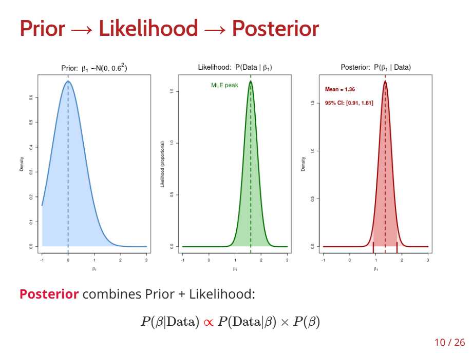
1. Prior beliefs → What we think before seeing data

2. Likelihood → How well different parameter values explain our data

3. Posterior distribution → Updated beliefs after seeing data

4. Practical interpretation → What these distributions tell us about our research questions

Bayesian Linear Regression

Likelihood: Defined from the regression model, which describes every independent observation yi as:

yi=β0+β1xi+ϵi,ϵi∼N(0,σ2)

same as yi∼N(β0+β1xi,σ2)

P(yi|β)=1√2πσ2exp(−(yi−β0−β1xi)22σ2)

Because we assume independence, the likelihood of the data y1,…,yn is the product of the likelihoods for each data point.

P(Data|β)=P(y1,…,yn|β)=n∏i=1P(yi|β)

Likelihood: yi∼N(β0+β1xi,σ2)

P(Data|β)=n∏i=1P(yi|β)=L(β|Data)

Prior distributions over parameters

• β1∼Normal(0,10) (slope prior)

• β0∼Normal(0,100) (intercept prior)

• σ∼Uniform(0,10) (error variance prior)

Posterior distribution: P(β|Data)∝P(Data|β)×P(β)

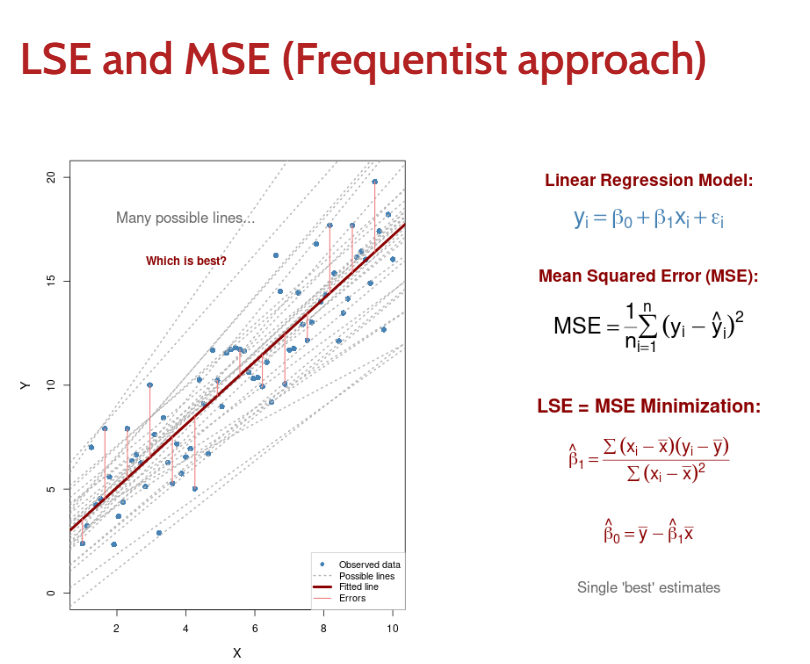
Frequentist approach Point Estimates to Distributions

Parameters have fixed (unknown) true values

• Provides a point estimate: ^β1=1.47

• Quantifies uncertainty through a confidence interval

  • A range of values, constructed from the data, that would contain the true parameter in a fixed proportion of repeated samples.

CI95%=[1.12,1.82]

"If we repeated this study many times, 95% of the confidence intervals would contain the true (fixed) parameter value."

Bayesian approach (point estimates to distributoins)

Parameters are random variables with distributions

• Specifies a full posterior distribution: P(β1|Data)∼Normal(1.47,0.182)

• Quantifies uncertainty through a credible interval

  • A range of values within which the parameter lies with a certain posterior probability, given the observed data.

P(1.12<β1<1.82|Data)=0.95

"Given our data, there is a 95% probability that the parameter lies in this interval."

Binomial Distribution

We have n independent trials, each with probability θ of success. How many successes X will we observe?

Binomial Distribution: X∼Binomial(n,θ)

P(X=k)=(nk)θk(1−θ)n−k

k=number of successes,n=number of trials θ=probability of success

Examples:

• Coin flips: n = 10 flips, θ = 0.5 (fair coin)

• Medical treatment: n = 50 patients, θ=??? (success rate)

• Survey responses: n = 100 people, θ=??? (proportions)

Binomial Likelihood function

The Binomial probability mass function already describes the likelihood of observing k successes in n trials.

P(X=k|n,θ)=(nk)θk(1−θ)n−k

As such, the Likelihood function L(θ|k,n)=P(X=k|n,θ) is:

P(X=k|n,θ)=(nk)θk(1−θ)n−k=L(θ|k,n)

Bernoulli Trials to Binomial Distribution

Key Insight: The Binomial distribution expresses the likelihood of observing k successes in n independent Bernoulli trials .

yi∼Bernoulli(θ)whereθ=P(yi=1)

• Each trial i has outcome yi∈{0,1} (failure or success)

• The complement rule dictates that P(yi=0|θ)=1−θ

As such, the probability of observing either yi=1 or yi=0 can be simply written as:

P(yi|θ)=θyi(1−θ)1−yi

Now, for a sequence of n independent Bernoulli trials:

• Observe sequence: y1,y2,…,yn where each yi∈{0,1}

Joint likelihood:

P(y1,y2,…,yn|θ)=n∏i=1P(yi|θ)=n∏i=1θyi(1−θ)1−yi=θ∑ni=1yi(1−θ)n−∑ni=1yi

We denote k=∑ni=1yi as the total number of successes, and the likelihood becomes:

P(y1,y2,…,yn|θ)=θk(1−θ)n−k

In order to express the likelihood in terms of the number of successes k, we need to account for all possible sequences of successes and failures.

• How many ways can we arrange k successes in n trials?

Example: n=3, k=2:

Possible sequences: {1,1,0},{1,0,1},{0,1,1} → 3 possible ways

The binomial coefficient (nk) is the number of distinct sequences (permutations) with k successes.

(nk)=n!k!(n−k)!

Binomial probability mass function

already describes the likelihood of observing k successes in n trials.

P(K=k|n,θ)=(nk)θk(1−θ)n−k=L(θ|k,n)

Rate estimation

We are often interested in estimating the rate parameter θ of a Binomial process formed by a sequence of independent binary trials (i.e., Bernoulli trials).

θ=???

Frequentist reference point: ^θMLE=kn

considering the Maximum Likelihood Estimator (MLE) for the parameter θ in the Binomial distribution.

Step 1: Derive the log-likelihood function (easier to work with)

L(θ|k,n)=(nk)θk(1−θ)n−k

ℓ(θ)=lnL(θ|k,n)=ln(nk)+kln(θ)+(n−k)ln(1−θ)

Step 2: To find the maximum, take the derivative and set to zerodℓdθ=kθ−n−k1−θ=0

Step 3: Solve for θkθ=n−k1−θ⇒k(1−θ)=(n−k)θ

k−kθ=nθ−kθ⇒k=nθ

⇒^θMLE=kn

The Maximum Likelihood Estimator for the Binomial rate ^θMLE is the sample proportion.

If we observed 7 successes in 10 trials, our best guess for θ is 710=0.7

frequentist approach

gives us a single point estimate: ^θMLE=kn=0.7

Bayesian approach What is the distribution of plausible values for θ?

1. Prior distribution: P(θ) - Specify initial beliefs and knowledge about θ

2. Likelihood: P(data|θ) - How well do different θ values explain our data?

3. Posterior distribution: P(θ|data)∝P(data|θ)×P(θ) - Combine prior and likelihood to get the full distribution of θ