macro chapter 10

intro to the problem of macroeconomic fluctuations

long-term equilibrium vs short-term fluctuations

• graph

long-term models

• long-term models could not explain any fluctuations in production

  • production was predetermined by input factors & technology determine fixed output

  • Solow model explains long-term growth, but no short-term fluctuations

  • Principle: every supply creates its own demand (classical economy)

  • Demand has not yet played a central role in production

long-run equilibrium

• GDP development fluctuates around the long-term equilibrium

  • economic cycles with periods of recession

  • economic cycles have different and unpredictable lengths

  • recession: usually 2 successive quarters of -ve GDP growth

  • unemployment, consumption and investment also fluctuate with GDP

  • okun's law: -ve relationship between unemployment & GDP

short vs long term view

• assumption: difference lies in the price adjustment

  • long-term: prices are flexible & adapt to changes

  • short-term: prices are fixed at given level

• consequence

  • economic policy measures have different effects in both

• intuition of content

  • if prices fail to adjust to changes, real variables of production must take over part of adjustment in short-term

  • price rigidity is common → companies only adjust prices 1-2 times per year

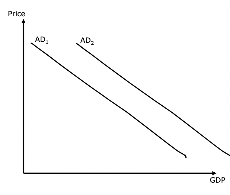
aggregated demand (AD)

• relationship between demand & the macroeconomic price level

• determines shape of AD cuve

3 ways to drive the AD curve

• from the quantity theory

• from the IS-LM model

• ad-hoc or intuitive

AD according to quantity theory

• quantity equation: M x V = P x Y

  • M = money supply

  • V = volume of money

• demand for money: M/P = kY

  • is proportional to production volume

  • there is -ve relationship between price level P and output Y

• intuition: if price level rises, a higher euro amount must be spent on each transaction, so production must fall

• change in money supply or interest rate, shifts AD curve

ad hoc derivation of aggregated demand

• as prices rise, consumption is postponed in favour of savings

• when prices fall, consumption pays off, & aggregate demand increases

• investments resulting from savings also increase total demand with Y = C + I + G → unclear if banks always pass on savings directly to investors

• if total demand changes irrespective of price, AD curve shifts

aggregated demand graph

• AD curve: -ve relationship between GDP + price

• right shift due to additional shift spending (G) and expansion of money supply (M)

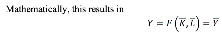
total supply in long-term

• quantity of goods produced depends on given quantity of input factors & production technology → fixed

• formula corresponds to long-term offer that is independent of price

• graph: vertical curve or line

• line above K,L,Y = fixed amount of that variable

total offer in the short-term

• assumption of fixed prices defined the short-term

• great simplification: all prices are fixed in the short term

• if price level is fixed → horizontal curve or line

• consequence → in short-term, only changes in supply can influence output level

  • supply shocks are cost shocks that lift the curve

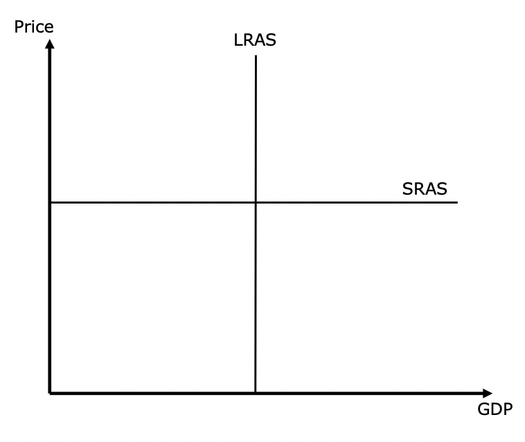
aggregated supply: 2 curves

1. aggregated supply in long-term: LRAS

   • long-run aggregated supply

   • vertical curve

2. aggregated offer in short-term: SRAS

   • short-run aggregated supply

   • horizontal curve

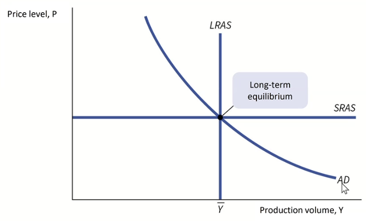
long-term equilibrium in AD-AS model

• in long-term, economy is at the intersection of long-term AS and AD curves

• as prices have adjusted to this level, the short-term aggregate supply curve also runs through this point

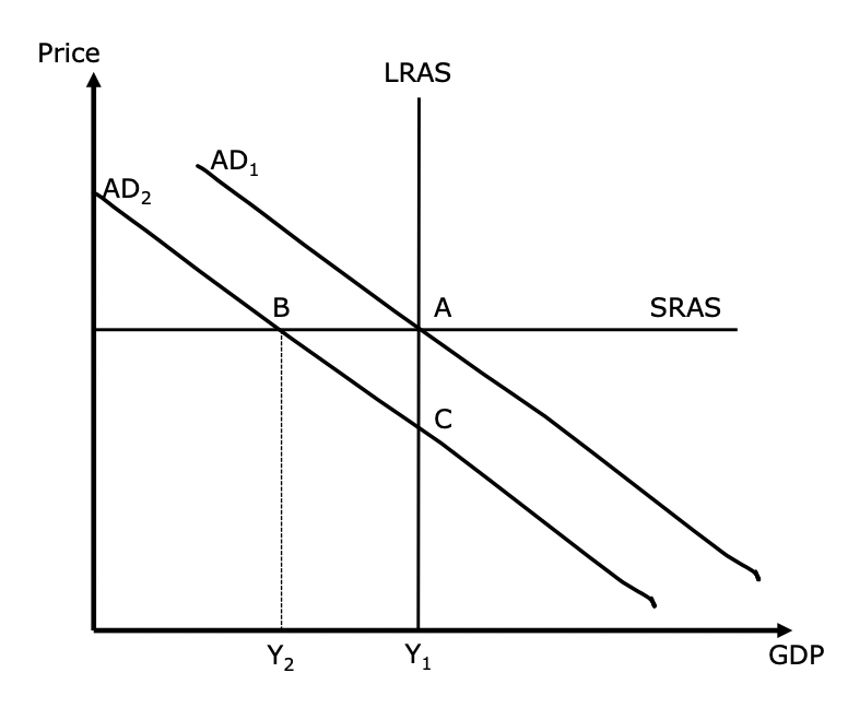
recession in AD-AS model

• demand shock shifts AD curve to the left

• in short term, the economy moves from equilibrium at point A to the new intersection point B of AD2 and SRAS

• if shock is permanent, economy will move from point B to long-term equilibrium at point C in long term

• if demand recovers in long-term, economy would move from point B back to the long-term equilibrium at point A

fiscal policy

• increase in government spending allows a rightward shift of the AD curve

• states can pay out ‘windfall money’ to the population to boost private consumption → AD curve shifts to the right

  • has a stabilising effect because population suffering from a drop in income is directly benefited

monetary policy

• by expanding the money supply, the central bank stimulates economy → right shift in AD curve

• reduction in money supply by central bank → left shift in AD curve

  • counteracts a +ve demand shock, but at the expense of the upswing

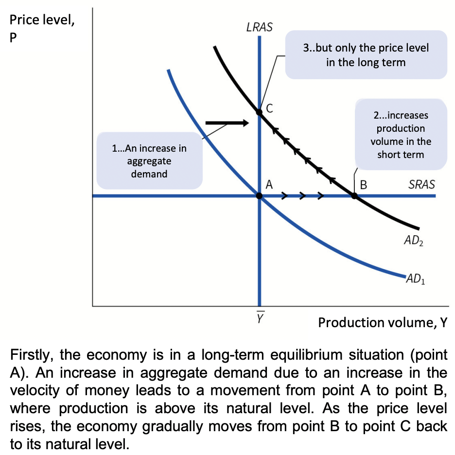
reaction of +ve demand shock

• +ve demand shock → AD curve shift right

• short-term upswing → slow down in long → prices rise

• if price stability is primary goal, the central bank should intervene and put brakes on the upswing

  • central bank could reduce money supply & try to bring the AD curve back to the initial situation

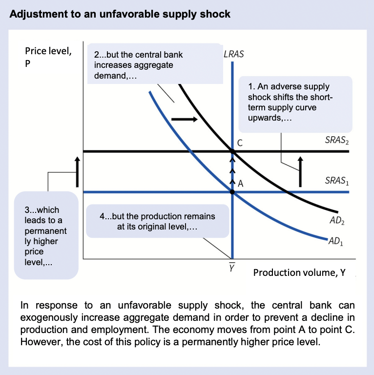
reaction to adverse supply shock

• cost shock increases production costs

  • oil price, delivery failures, gas crisis

• SRAS curve shifts upwards

• to prevent a recession with a simultaneous rise in prices (stagflation), AD curve can be shifted to right through monetary or fiscal policy

• decline in income can be prevented at the expense of a long-term rise in prices