AP Statistics Midterm Flashcards
1/53
Earn XP
Description and Tags
Name | Mastery | Learn | Test | Matching | Spaced | Call with Kai | Chat |
|---|
No analytics yet
Send a link to your students to track their progress
54 Terms
Random
Unpredictable in the short run and predictable in the long run.
Law of Large Numbers (a.k.a. Law of Averages):
As we observe more and more repetitions of any chance process, the proportion of times that a specific outcome occurs approaches its probability.
Informally, outcomes balance out in the long run.
A misguided belief is outcomes balance in the short run.
Probability:
A number between 0 and 1 that describes the proportion of times an outcome would occur in a very long series of repetitions.
Simulation
The imitation of chance behavior using a model that reflects the situation.
The Simulation Process
Describe how to use a chance process to imitate one trial, and what will be recorded.
Perform many trials.
Use the results to answer the question.
Sample space:
the set of all possible outcomes
Probability Model:
A two-part description of chance process. It includes:
the sample space; and
the probability for each outcome
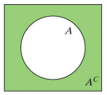
Complement
The complement of an event is all the outcomes not in that event. That is, the complement of A is “all events other than A” and is notated A^C (or A bar).
The complement rule says that P(A^C)=1-P(A)
For a probability model to be valid:
All outcomes are represented.
The sum of the probabilities is 1
(with each probability between 0 and 1)
Mutually exclusive
There are no common outcomes between two events
The addition rule
P(A or B)=P(A)+P(B) is limited to events that are mutually
exclusive (having no common outcomes).
Generalised addition rule
A generalized addition rule for probability is P(A or B)=P(A)+P(B)-P(A and B) and is valid for any two events.
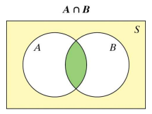
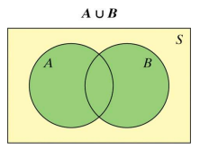
Venn Diagram
A Venn diagram consists of one or more circles surrounded by a rectangle. Each circle represents an event. The region inside the rectangle represents the sample space.
Intersection
The intersection of A and B is notated A ∩ B and is all outcomes in both A and B. (A and B)
Union
The union of A and B is notated A ∪ B and is all outcomes in either event A or B. (A or B)
Conditional Probability
The probability that one event happens given that another event is known to have happened is a conditional probability. The conditional probability that event B happens given that event A has happened is denoted P(A|B)
P(A|B) = P(A and B) / P(B)
Independence
Events are independent when knowing that one event has occurred does not change the probability of the other event. That is, events A and B are independent if:
P(A|B) = P(A) and P(B|A) = P(B)
Tree Diagram
A tree diagram shows the sample space of a chance process involving stages. The probability of each outcome is shown on the corresponding branch of the tree. All probabilities after the first stage are conditional probabilities.
Can two events be mutually exclusive and independent?
No!!!
Random Variable
A random variable is numerical variable whose value depends on the outcome of a chance experiment. A numerical value (probability) is associated with each outcome of the chance experiment.
Discrete random variable
A random variable is discrete if its possible values are isolated along the number line. The number of patients is an example of a discrete random variable.
Continuous random variable
A random variable is continuous if its possible values are all points in an interval on the number line. Body temperature of each patient is an example of a continuous random variable.
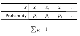
Probability distribution of a discrete random variable
The probability distribution of a discrete random variable, X, lists all the outcomes, xi , and the associated probabilities. This can be shown using a histogram or table.
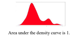
Probability distribution of a continuous random variable
The probability distribution of a continuous random variable, X, is commonly shown using a density curve. This may include the normal curve.
Expected value
The mean of a random variable, X, is commonly referred to as the expected value.
The expected value is not always a member of X.
The expected value of X can be notated as E(X) or ux
The expected value should include units.
For discrete variables, the expected value is:
E(X) = ux = x1p1 + x2p2 + x3p3 + …
Effect of Adding (or Subtracting) a random variable by a
Measures of center and location increase by a
Measures of spread are unchanged
Shape is unchanged
Effect of Multiplying (or Dividing) a random variable by b
Measures of center and location are multiplied (or divided) by b
Measures of spread are multiplied (or divided) by b
Shape is unchanged
If X and Y are any two random variables, then:
ux+y = ux + uy
ux-y = ux - uy
If X and Y are independent random variables, then:
o²x+y = o²x + o²y
o²x-y = o²x + o²y
Binomial Setting
A binomial setting arises when we perform n independent trials of the same chance process and count the number of times that a particular outcome (called a “success”) occurs.
As a convention:
the number of trials is n
the probability of success for one trial is p
the number of desired successes is k
Characteristics of a binomial setting:
Use the acronym, BINS:
Binary: The outcome of each trial can be classified as “success” or “failure.”
Independent: The outcome of one trial does influence the outcome of any other trial.
Number: The number of trials is fixed in advance.
Same probability: There is the same probability of success on each trial.
Binomial distribution
The number of successes is a random variable, X. The probability distribution of X is known as a binomial distribution and is notated X~B(n, p)
P(X=k) = nCk(p)^k(1-p)^(n-k)
ux = np
ox = √(np(1-p))
10% Condition
Sampling Without Replacement (a.k.a. The 10% Condition):
A binomial distribution can still be used even when the independent condition is not met if the sample of size, n, does not exceed 10% of the population size, N. That is,
n <= 0.1N
Large Counts Condition
A binomial distribution can be modelled by a normal distribution when the Large Counts Condition is satisfied. That is,
np >= 10 and n(1-p) >= 10
Geometric Setting
Although very similar to the binomial setting, the number of trials not being fixed is the fundamental difference. The trials continue until the first success.
The probability of a geometric variable requiring k trials is:
P(X=k) = (1-p)^(k-1) * (p)
If X is a geometric random variable, then:
ux = E(x) = 1/p
ox = √(1-p)/p
Parameter
A number describing the population is a parameter.
Statistic
A number describing a sample is a statistic.
Point estimator
A sample statistic is sometimes called a point estimator of the corresponding population parameter because the estimate is a single point on the number line.
Sampling variability
Sampling variability is the phenomenon that different random samples of the same size from the same population produce different values for a statistic.
Sampling Distribution:
the distribution formed by the values of a sample statistic for every possible sample of size n.
Population distribution
The population distribution gives the values of the variable for all individuals in the population.
Distribution of sample data
The distribution of sample data shows the values of the variable for the individuals in a sample.
Unbiased estimator
A statistic is an unbiased estimator if the mean of its sampling distribution is equal to the true value of the parameter. That is,
u(sample statistic) = Parameter
p-hat and x-bar are unbiased estimators of p and u , respectively
Sample size and variability
The variability of a sampling distribution is primarily determined by the size of the sample. Larger samples have smaller variability. While larger samples reduce variability, they do not eliminate bias. To decide which estimator to use when there are several reasonable choices, consider both bias and variability.
Accurate
Close to the actual value
Precise
Consistent
Sampling distribution of sample proportion, p-hat
The sampling distribution of the sample proportion p̂describes the distribution of values taken by the sample proportion p̂ in all possible samples of the same size from the same population.
Shape of the sampling distribution of p-hat
When n is small and p is close to 0, the distribution of p̂ is skewed to the right
When n is small and p is close to 1, the distribution of p̂ is skewed to the left
When n is small and p is close to 0.5, the distribution of p̂ is symmetric
approximately normal as n increases, but depends on n and p
normal conditions remain when np >= 10 and n(1-p) >= 10
Center of the sampling distribution of p-hat
u pˆ = p ( pˆ is an unbiased estimator of p)
Variability of the sampling distribution of p-hat
dispersion decreases as n increases
op = √(p(1-p)/n)
Trials must be independent or the 10% condition must be met
Sampling Distribution of p-hat1 - p-hat2
The sampling distribution of p̂1 − p̂2 is approximately Normal if the Large Counts condition is met for both samples
The mean is
The standard deviation is op̂1 − p̂2 = √(op-hat1²+op-hat2²); but relies on the 10% condition for both samples. [Must establish 10% condition if sampling without replacement]
Sampling distribution of x-hat
The sampling distribution of x is similar to that of the sample proportion pˆ
The sample mean, x , is an unbiased estimator of the population mean, μ.
The values of x are less spread out for larger samples.
The standard deviation of the sampling distribution is o/√n if independence or the 10% condition is met
Sampling from a normal population
If X is normally distributed according to N(u, o), then the sampling distribution of x is normally distributed according to N(u, o/√n) (if independence or the 10% condition is met).
The Central Limit Theorem
The distribution of x from any population is approximately normal if n is large*.
* Conventionally, ‘large’ is n >= 30 ; though for populations closer to normal, a smaller sample may suffice.