Unit 6 - Discrete-time Signals and Systems

Biological Signals

generally CT; they are routinely sampled to yield discrete-time (DT) signals to facilitate signal analysis via computers

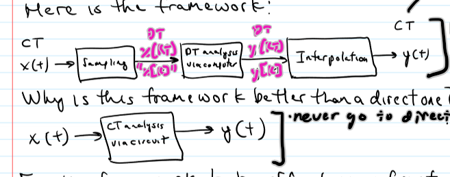
better than one below because it is recomfigureable (no component error; less costly, faster, and easier; more accurate); info can’t be lost in the sampling process and equivalent to saying that x(t) can be recovered from its samples (x[k])

Info in x(t) can’t be lost in the sampling process

intuitively, 2 conditions should be met for the answer to be yes → x(t) must have smoothness and the sampling must be fast enough

Shannon’s Sampling Theorem

CT signal, x(t), that is bandlimited frequency to BHz or 2piB rad/sec; x(t) can be exactly recovered from its sample x(k)=x(kt) provided that; Fs (sampling frequency) = 1/T (sampling interval) > 2B; 

Proof of Shannon’s Sampling Theorem

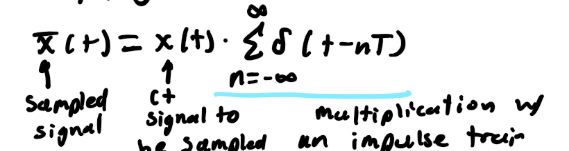
a signal can be sampled in time by multiplying it by an impulse train

Examples

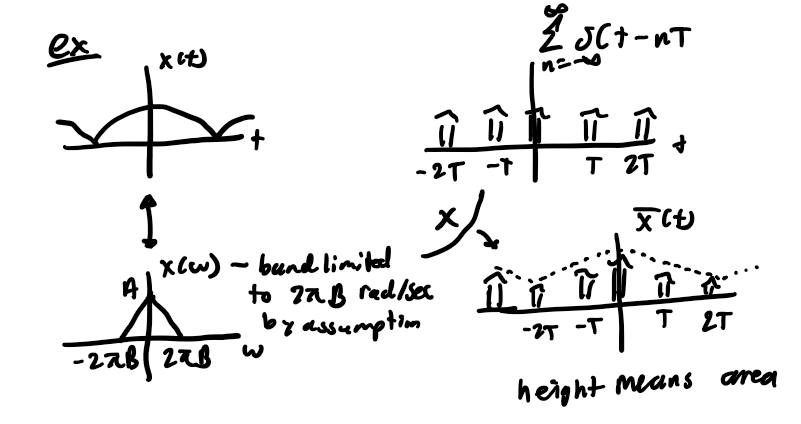
What is happening in the frequency domain?

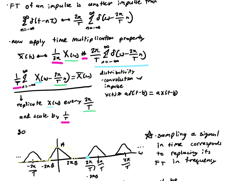
FT of an impulse is another impulse train; now apply time multiplication property; use distributivity and convolution w/ impulse; replicate X(w) every (2pi/T) and scale by (1/T); to reconstruct x(t) from xbar(t), X(w) should be recoverable from Xbar(w); this is possible if there is no overlap between successive cycles in Xbar(w) → X(w) can be recovered by a low pass filter; for no overlap to occur (2pi/T - 2piB >  2piB) so 1/T > 2B

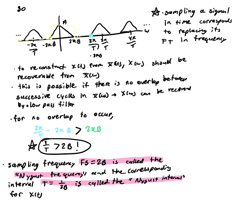
Nyguist Frequency

sampling frequency Fs = 2B

Nyguist Interval

interval T = 1/2B

Nyguist Interval in Plain Language

process of reconstructing a CT signal from its samples

Interpolation

the process of reconstructing a CT signal from its samples, amounts to lowpass filtering

What happens in the time-domain?

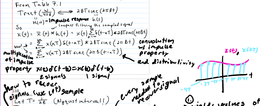
x(t) = xbar(t)*h(t) = sum of - infinity to infinity of x(nT)*sinc(2piB(t-nT)) → interpolation formula

Interpolation Formula yields values of x(t)

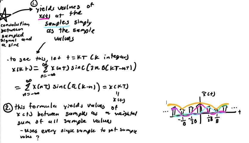
1. yields values of x(t) at the samples simply as the sample values

2. this formula yields values of x(t) between samples as a weighted sum of all sample values (uses every single single to get sample values??)

x(t) at the samples simply as the sample values

let t=kT (k integar): x(kT) = sum of - infinity to infinity of x(nT)*sinc(pi(k-n)) = x(kT) = x(t)

2 Practical Difficulties w/ Interpolation Formula

1. if signal is sampled just above Nyguist rate (ws = 2pi/T = 4piB) then x(t) can only be recovered w/ an ideal LPF, which is not physically realizable

2. sampling theorem assumes that x(t) is bandlimited but all practical signals are time limited

Oversampling

make sample significantly greater than the Nyguist rate (triangle further apart) so well above 4piB

Practical Filter

w/ a finite width transition band could be used for interpolation; Fx > 2B is thus a theoretical limit

Timing-Scaling Property

implies that signals can’t be both of finite duration and bandlimited

What happens when practical signals that aren’t bandlimited, are sampled?

even if ideal interpolation were possible, the reconstructed signal would be unsatisfactory

Unsatisfactory because

loss of high frequency info, x(w) above pi/T rad/sec (losing tails) and reappearance of this “tail” within +- rad/sec (tails switch, called “aliasing/spectra folding”)

Aliasling/Spectra folding

when high frequency impersonate low frequencies; can be fixed with pre-filtering

Pre-filtering/anti-aliasfiltering

apply a LPF, x(t), prior to sampling to make it as bandlimited as possible

Summary

theory - bandlimited to BHz, Fs > 2B convolution w/ sinc

practice - LPF, x(t), to B before sampling Fs »2B

Sampling a CT Sinusoid

let x(t)=cos(wt) be sampled at T sec intervals; x[k]=x(kT)=cos(wkT)=cos(wTk) so x[k]=cos(omega k), omega=wT (normalized frequency) in rads

CT vs DT Sinusoids

CT - x(t) and unique for each w

DT - x[k] and not unique for each u

DT Sinusoid

of frequency, omega, is indistinguishable from a DT sinusoid of frequency, omega +- an integar of multiple 2pi; so can be expressed w/ omega between +- pi; since cos(omega k)=cos(-omega k) any real of this can be expressed w/ omega between 0 + pi; 0 is lowest frequency and pi is the highest

CT Sinusoid

must be sampled at a rate greater than 2 samples/cycle to avoid alaising

DT Signals

x[k]; defined only at integar values of time (t); has properties and special signals

DT Signal Properties

periodic/aperiodic (periodic if x[k]=x(k+No) for all k and integar No)

uni/multidimensional

energy/power/neither (integration in CT corresponds to summing in DT)

deterministic/stochasic 

Special DT Signal

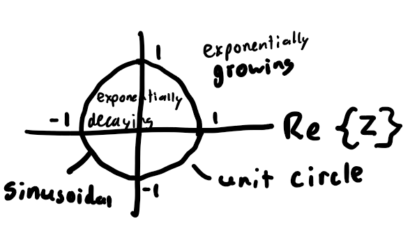
exponentially varying sinusoids (gamma^k)

|gamma| < 1: decays as k → infininty

|gamma| > 1: grows as k → infinity

|gamma| = 1: oscillates as k → infinity

these can be visualized in the complex (z-plane) 

Analogies Between s-plane and z-plane

S: based on e^(st) where s is in cartesian coordinates

Z: based on gamma^k wheer gamma is in polar coordinates

S (LHP) ←> Z (within unit circle)

S (RHP) ←> Z (outside unit circle)

S (jw-axis) ←> Z (on unit circle)

Singularity Signals

entirely analogous to their CT counterparts but simpler; ex. DT step fcn and DT impulse fcn; summming plays a role of integrating in DT and differencing plays role of differentiating in DT

DT System Properties

same as CT

Time-domain Analysis of DT LTI Systems

very similar to CT but convolution is now a sum

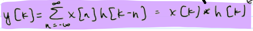
Example

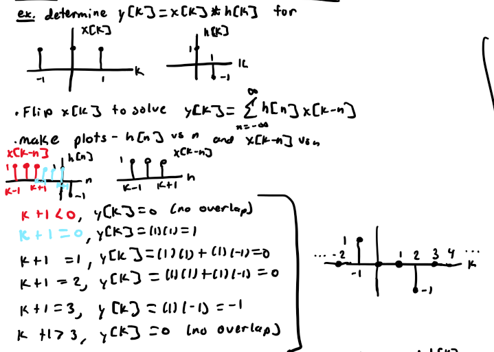
y[k] is N + M -1 Samples in Duration

in general, if x[k] is N samples in duration and h[k] is M samples in duration

LCCDEs

differential equations are difference equations in DT: a2 y[k-2] + a1 y[k-1] + ao y[k] = b1 x[k-1] + b2 x[k]; can be solved analogously (homogenous + particular or initial conditions or by recursion/iteration)

LCCDEs - Homogenous + Particular

yh[k] + yp[k]

LCCDEs - Initial Conditions

yZIR[k] + yZSR[k]

LCCDEs - Recursion/Iteration

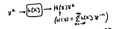
How to determine the output of DT LTI systems using multiplication and not convolution?

represent DT signals as sums of exponentially-varying sinusoids and invoke lineraity

Z-Transform (ZT) Analysis of DT Signals and LTI Signals

a frequency-domain technique in which DT signals are representaed as sums of exponentially-varying sinusoids

Unilateral ZT of a DT Signal, x[k], is this complex form

x(z) = sum from k=0 to infinity of x[k]*z^(-k); z is a complex # for which the finite sum exists; exists for DT signals that grow no faster than an exponential

Z

a complex # for which the finite sum exists

ZT exists for DT Signals when

signals grow no faster than an exponential

Z^k instead of e^(zk)

“causal signals” that have a ZT have ROC outside some circle in the z-plane

Inverse ZT Equation

likewise a contour integral so PFE should instead be used for inverse transforming

ZT Properties

time convolution and right shift

Time Convolution

if x[k] ←> X(z) and h[k] ←> H(z), then x[k]*h[k] ←> x(z) H(z); useful for solving ZSR

Right Shift

if x[k] ←> X(z) then, x[k-1] ←> z^(-1) X(z) + x[-1] then x[k-2] ←> z^(-1) X(z) + x[-1] + x[-2]; useful for solving LCCDes (differences)

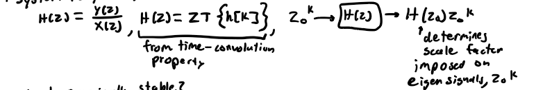
System Function, H(z), of a DT LTI System Parallels H(s)

Example

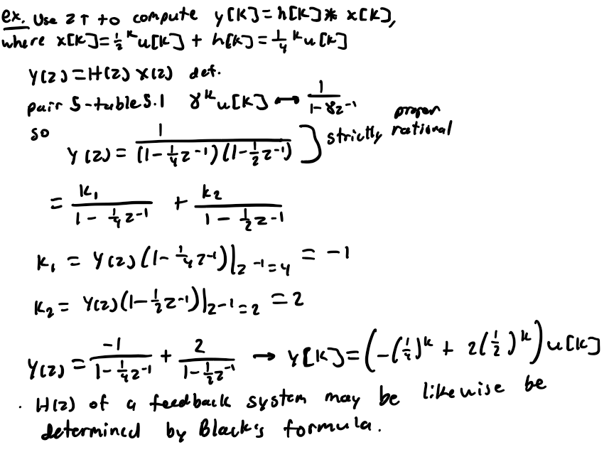
H(z) of a Feedback System

may be likewise be determined by Black’s formula

Frequency Response

input: x[k] = gamma^k (exponentially-varying sinusoid) where gamma = 1; y[k] = H(e^(jomegao))*e^(j omega k); Acos(omegao K + phi) → H(z) → A|H(e^jomego)|*cos(omegaok + phi + angle of H(e^jomegao))

H(e^(j omega)) as a fcn of omega

the frequency response of a DT LTI system

H(e^jomega)

evaulating H(z) around the unit circle in the z-plane; always a periodic fcn of omega w/ period 2pi (bc e^(jomega) = e^(j(omega + 2pi))

Frequencies in DT

lowest: 0

highest: pi

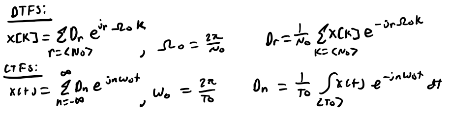
Discrete-Time Fourier Series (DTFS)

same as CTFS w/ 1 difference; since frequency range in DT is 2pi and harmonics are separated in frequency in omega naught = 2pi/No so only No harmonic

DTFS Line Spectra

(Dr vs r) will be periodic w/ period No and thus need only be plotted over -No/2 <= r < No/2

DTFS vs CTFS

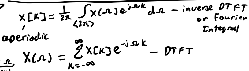
DTFT for Representing Aperiodic Signals

a continum of frequency over 2pi interval for needed; X(omega) is a periodic fcn of omega w/ period 2pi

DTFT Spectra

X(omega) vs omega; continous plot but signal discrete plotted over -pi <= omega < omega

If x[k] real then

magnitude spectrum (|x(omega)| vs omega) and phase spectra (angle of x(omega) vs omega) will be even and odd respectively

What signals does DTFT exist for?

absolutely and square summable DT signals; power signals if impulse(omega) allowed in x(omega); DNE for growing signals

DTFT and ZT

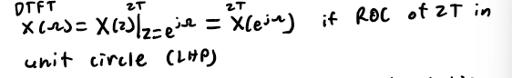
DTFT of h[k]

of a causal, stable system is the frequency response

DTFT Properties

y[k] = h[k]*x[k] ←> Y(omega) = H(omega)X(omega) but, like the LT, the ZT is perferred for system analysis

Example of Impulse response

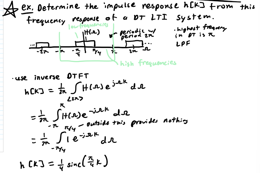
Ideal LPF is not what?

physically realizable

Practical Approach to Filter Design

windowing the sinc

CT vs DT

CT: t - continous, integrals, derivatives, e^st (jw-axis), w: - infinity → infinity

DT: k - integar, sums, differences, gamma^k (unit circle), omega (- pi → pi) (periodic)