normal distribution

normal distribution

aka bell curve, a continuous probability distribution that can be used to model many naturally occuring scenarios such as height

ND notation

X~N(μ, σ²)

where variable X follows a normal distribution with mean μ and variance σ²

ND characteristics

-bell-shaped curve with asymptotes at each end

-symmetrical (mean = median = mode)

-total area under curve equal to 1 (as area under any section equal to probability of that section)

-has P(X = a) = 0 for any a (as it is a continuous distribution with infinite possible values for X)

-points of inflection at μ ± σ

mean and variance effects on ND curves

if the mean changes the graph is translated horizontally, if the variance changes the graph is stretched or squashed vertically

finding probabilities for normal distributions

for P(X < n) and X~N(μ, σ²)

use the normal cumulative distribution function on your calculator, entering the mean and the standard deviation, and n as the upper bound with an extremely small value as a lower bound (at least 5 standard deviations from the mean, can be negative)

bounds reverse for P(X>a) but this function is less common on calculators, 1 - P(X<a) is usually used instead

ND variable probabilities

-approximately 68% of the data lies within one standard deviation of the mean

-95% of the data lies within two standard deviations of the mean

-99.7% of the data lies within three standard deviations of the mean

inverse ND function

inverse normal function on a calculator finds the value of a such that P(X < a) = p

you will need to enter the area/tail (p), the mean and the standard deviation

the value of a such that P(x > a) = p is

standard normal distribution

normal distribution with mean 0 and standard deviation 1- Z~N(0, 1!)

useful when the mean or variance of a ND is unknown as any ND can be coded as a standard ND

Z formula

converts a random variable X~N(μ, σ²) to a standard normal variable

Z = (X - μ)/σ²

Φ(a) is equivalent notation to P(Z < a)

approximating a binomial distribution

if n is large and p is close to 0.5 (as the normal distribution is symmetrical) the binomial distribution X~B[n,p] can be approximated by the normal distribution X~N(μ, σ²) where:

-μ = np

-σ² = np(1-p)

this method is inaccurate due to BDs' discrete nature in contrast to ND’s continuous nature, the continuity correction is used to remedy this

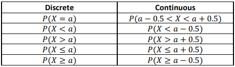
continuity correction

0.5 is added or subtracted from the approximation(s) given

hypothesis testing with the normal distribution

for a random sample of size n taken from a random variable X~N(μ, σ²), the sample mean X̄ is normally distributed with X̄~N(μ, σ²/n)

this information can be used on a sample of a normal distribution to see whether the mean from the sample is significant enough to reject the null hypothesis